Abstract
Most air pollution research has focused on assessing the urban landscape effects of pollutants in megacities, little is known about their associations in small- to mid-sized cities. Considering that the biggest urban growth is projected to occur in these smaller-scale cities, this empirical study identifies the key urban form determinants of decadal-long fine particulate matter (PM2.5) trends in all 626 Chinese cities at the county level and above. As the first study of its kind, this study comprehensively examines the urban form effects on air quality in cities of different population sizes, at different development levels, and in different spatial-autocorrelation positions. Results demonstrate that the urban form evolution has long-term effects on PM2.5 level, but the dominant factors shift over the urbanization stages: area metrics play a role in PM2.5 trends of small-sized cities at the early urban development stage, whereas aggregation metrics determine such trends mostly in mid-sized cities. For large cities exhibiting a higher degree of urbanization, the spatial connectedness of urban patches is positively associated with long-term PM2.5 level increases. We suggest that, depending on the city’s developmental stage, different aspects of the urban form should be emphasized to achieve long-term clean air goals.
Introduction
Air pollution represents a prominent threat to global society by causing cascading effects on individuals1, medical systems2, ecosystem health3, and economies4 in both developing and developed countries5,6,7,8. About 90% of global citizens lived in areas that exceed the safe level in the World Health Organization (WHO) air quality guidelines9. Among all types of ecosystems, urban produce roughly 78% of carbon emissions and substantial airborne pollutants that adversely affect over 50% of the world’s population living in them5,10. While air pollution affects all regions, there exhibits substantial regional variation in air pollution levels11. For instance, the annual mean concentration of fine particulate matter with an aerodynamic diameter of less than 2.5 \(\upmu\mathrm{m}\) (PM2.5) in the most polluted cities is nearly 20 times higher than the cleanest city according to a survey of 499 global cities12. Many factors can influence the regional air quality, including emissions, meteorology, and physicochemical transformations. Another non-negligible driver is urbanization—a process that alters the size, structure, and growth of cities in response to the population explosion and further leads to lasting air quality challenges13,14,15.
With the global trend of urbanization16, the spatial composition, configuration, and density of urban land uses (refer to as urban form) will continue to evolve13. The investigation of urban form impacts on air quality has been emerging in both empirical17 and theoretical18 research. While the area and density of artificial surface areas have well documented positive relationship with air pollution19,20,21, the effects of urban fragmentation on air quality have been controversial. In theory, compact cities promote high residential density with mixed land uses and thus reduce auto dependence and increase the usage of public transit and walking21,22. The compact urban development has been proved effective in mitigating air pollution in some cities23,24. A survey of 83 global urban areas also found that those with highly contiguous built-up areas emitted less NO222. In contrast, dispersed urban form can decentralize industrial polluters, improve fuel efficiency with less traffic congestion, and alleviate street canyon effects25,26,27,28. Polycentric and dispersed cities support the decentralization of jobs that lead to less pollution emission than compact and monocentric cities29. The more open spaces in a dispersed city support air dilution30. In contrast, compact cities are typically associated with stronger urban heat island effects31, which influence the availability and the advection of primary and secondary pollutants32.
The mixed evidence demonstrates the complex interplay between urban form and air pollution, which further implies that the inconsistent relationship may exist in cities at different urbanization levels and over different periods33. Few studies have attempted to investigate the urban form–air pollution relationship with cross-sectional and time series data34,35,36,37. Most studies were conducted in one city or metropolitan region38,39 or even at the country level40. Furthermore, large cities or metropolitan areas draw the most attention in relevant studies5,41,42, and the small- and mid-sized cities, especially those in developing countries, are heavily underemphasized. However, virtually all world population growth43,44 and most global economic growth45,46 are expected to occur in those cities over the next several decades. Thus, an overlooked yet essential task is to account for various levels of cities, ranging from large metropolitan areas to less extensive urban area, in the analysis.
This study aims to improve the understanding of how the urban form evolution explains the decadal-long changes of the annual mean PM2.5 concentrations in 626 cities at the county-level and above in China. China has undergone unprecedented urbanization over the past few decades and manifested a high degree of heterogeneity in urban development47. Thus, Chinese cities serve as a good model for addressing the following questions: (1) whether the changes in urban landscape patterns affect trends in PM2.5 levels? And (2) if so, do the determinants vary by cities?
Data
City boundaries
Our study period spans from the year 2000 to 2014 to keep the data completeness among all data sources. After excluding cities with invalid or missing PM2.5 or sociodemographic value, a total of 626 cities, with 278 prefecture-level cities and 348 county-level cities, were selected. City boundaries are primarily based on the Global Rural–Urban Mapping Project (GRUMP) urban extent polygons that were defined by the extent of the nighttime lights48,49. Few adjustments were made. First, in the GRUMP dataset, large agglomerations that include several cities were often described in one big polygon. We manually split those polygons into individual cities based on the China Administrative Regions GIS Data at 1:1 million scales50. Second, since the 1978 economic reforms, China has significantly restructured its urban administrative/spatial system. Noticeable changes are the abolishment of several prefectures and the promotion of many former county-level cities to prefecture-level cities51. Thus, all city names were cross-checked between the year 2000 and 2014, and the mismatched records were replaced with the latest names.
PM2.5 concentration data
The annual mean PM2.5 surface concentration (micrograms per cubic meter) for each city over the study period was calculated from the Global Annual PM2.5 Grids at 0.01° resolution52. This data set combines Aerosol Optical Depth retrievals from multiple satellite instruments including the NASA Moderate Resolution Imaging Spectroradiometer (MODIS), Multi-angle Imaging SpectroRadiometer (MISR), and the Sea-Viewing Wide Field-of-View Sensor (SeaWiFS). The global 3-D chemical transport model GEOS-Chem is further applied to relate this total column measure of aerosol to near-surface PM2.5 concentration, and geographically weighted regression is finally used with global ground-based measurements to predict and adjust for the residual PM2.5 bias per grid cell in the initial satellite-derived values.
Human settlement layer
The urban forms were quantified with the 40-year (1978–2017) record of annual impervious surface maps for both rural and urban areas in China47,53. This state-of-art product provides substantial spatial–temporal details on China’s human settlement changes. The annual impervious surface maps covering our study period were generated from 30-m resolution Landsat images acquired onboard Landsat 5, 7, and 8 using an automatic “Exclusion/Inclusion” mapping framework54,55. The output used here was the binary impervious surface mask, with the value of one indicating the presence of human settlement and the value of zero identifying non-residential areas. The product assessment concluded good performance. The cross-comparison against 2356 city or town locations in GeoNames proved an overall high agreement (88%) and approximately 80% agreement was achieved when compared against visually interpreted 650 urban extent areas in the year 1990, 2000, and 2010.
Control variables
To provide a holistic assessment of the urban form effects, we included control variables that are regarded as important in influencing air quality to account for the confounding effects.
Four variables, separately population size, population density, and two economic measures, were acquired from the China City Statistical Yearbook56 (National Bureau of Statistics 2000–2014). Population size is used to control for the absolute level of pollution emissions41. Larger populations are associated with increased vehicle usage and vehicle-kilometers travels, and consequently boost tailpipes emissions5. Population density is a useful reflector of transportation demand and the fraction of emissions inhaled by people57. We also included gross regional product (GRP) and the proportion of GRP generated from the secondary sector (GRP2). The impact of economic development on air quality is significant but in a dynamic way58. The rising per capita income due to the concentration of manufacturing industrial activities can deteriorate air quality and vice versa if the stronger economy is the outcome of the concentration of less polluting high-tech industries. Meteorological conditions also have short- and long-term effects on the occurrence, transport, and dispersion of air pollutants59,60,61. Temperature affects chemical reactions and atmospheric turbulence that determine the formation and diffusion of particles62. Low air humidity can lead to the accumulation of air pollutants due to it is conducive to the adhesion of atmospheric particulate matter on water vapor63. Whereas high humidity can lead to wet deposition processes that can remove air pollutants by rainfall. Wind speed is a crucial indicator of atmospheric activity by greatly affect air pollutant transport and dispersion. All meteorological variables were calculated based on China 1 km raster layers of monthly relative humidity, temperature, and wind speed that are interpolated from over 800 ground monitoring stations64. Based on the monthly layer, we calculated the annual mean of each variable for each year. Finally, all pixels falling inside of the city boundary were averaged to represent the overall meteorological condition of each city.
Methods
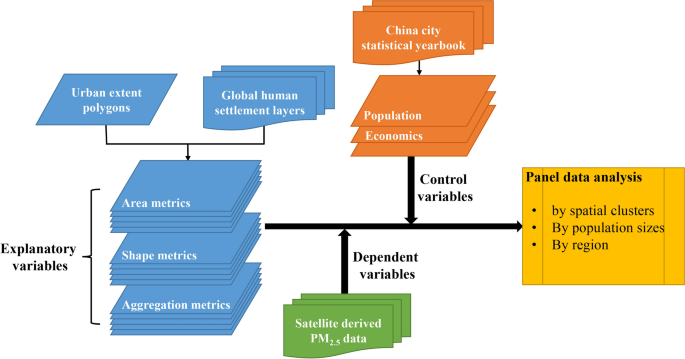
Considering the dynamic urban form-air pollution relationship evidenced from the literature review, our hypothesis is: the determinants of PM2.5 level trends are not the same for cities undergoing different levels of development or in different geographic regions. To test this hypothesis, we first categorized city groups following (1) social-economic development level, (2) spatial autocorrelation relationship, and (3) population size. We then assessed the relationship between urban form and PM2.5 level trends by city groups. Finally, we applied the panel data models to different city groups for hypothesis testing and key determinant identification (Fig. 1).
Calculation of urban form metrics
Based on the previous knowledge65,66,67, fifteen landscape metrics falling into three categories, separately area, shape, and aggregation, were selected. Those metrics quantify the compositional and configurational characteristics of the urban landscape, as represented by urban expansion, urban shape complexity, and compactness (Table 1).
Area metrics gives an overview of the urban extent and the size of urban patches that are correlated with PM2.520. As an indicator of the urbanization degree, total area (TA) typically increases constantly or remains stable, because the urbanization process is irreversible. Number of patches (NP) refers to the number of discrete parcels of urban settlement within a given urban extent and Mean Patch Size (AREA_MN) measures the average patch size. Patch density (PD) indicates the urbanization stages. It usually increases with urban diffusion until coalescence starts, after which decreases in number66. Largest Patch Index (LPI) measures the percentage of the landscape encompassed by the largest urban patch.
The shape complexity of urban patches was represented by Mean Patch Shape Index (SHAPE_MN), Mean Patch Fractal Dimension (FRAC_MN), and Mean Contiguity Index (CONTIG_MN). The greater irregularity the landscape shape, the larger the value of SHAPE_MN and FRAC_MN. CONTIG_MN is another method of assessing patch shape based on the spatial connectedness or contiguity of cells within a patch. Larger contiguous patches will result in larger CONTIG_MN.
Aggregation metrics measure the spatial compactness of urban land, which affects pollutant diffusion and dilution. Mean Euclidean nearest-neighbor distance (ENN_MN) quantifies the average distance between two patches within a landscape. It decreases as patches grow together and increases as the urban areas expand. Landscape Shape Index (LSI) indicates the divergence of the shape of a landscape patch that increases as the landscape becomes increasingly disaggregated68. Patch Cohesion Index (COHESION) is suggestive of the connectedness degree of patches69. Splitting Index (SPLIT) and Landscape Division Index (DIVISION) increase as the separation of urban patches rises, whereas, Mesh Size (MESH) decreases as the landscape becomes more fragmented. Aggregation Index (AI) measures the degree of aggregation or clumping of urban patches. Higher values of continuity indicate higher building densities, which may have a stronger effect on pollution diffusion.
The detailed descriptions of these indices are given by the FRAGSTATS user’s guide70. The calculation input is a layer of binary grids of urban/nonurban. The resulting output is a table containing one row for each city and multiple columns representing the individual metrics.
Division of cities
Division based on the socioeconomic development level
The socioeconomic development level in China is uneven. The unequal development of the transportation system, descending in topography from the west to the east, combined with variations in the availability of natural and human resources and industrial infrastructure, has produced significantly wide gaps in the regional economies of China. By taking both the economic development level and natural geography into account, China can be loosely classified into Eastern, Central, and Western regions. Eastern China is generally wealthier than the interior, resulting from closeness to coastlines and the Open-Door Policy favoring coastal regions. Western China is historically behind in economic development because of its high elevation and rugged topography, which creates barriers in the transportation infrastructure construction and scarcity of arable lands. Central China, echoing its name, is in the process of economic development. This region neither benefited from geographic convenience to the coast nor benefited from any preferential policies, such as the Western Development Campaign.
Division based on spatial autocorrelation relationship
The second type of division follows the fact that adjacent cities are likely to form air pollution clusters due to the mixing and diluting nature of air pollutants71, i.e., cities share similar pollution levels as its neighbors. The underlying processes driving the formation of pollution hot spots and cold spots may differ. Thus, we further divided the city into groups based on the spatial clusters of PM2.5 level changes.
Local indicators of spatial autocorrelation (LISA) was used to determine the local patterns of PM2.5 distribution by clustering cities with a significant association. In the presence of global spatial autocorrelation, LISA indicates whether a variable exhibits significant spatial dependence and heterogeneity at a given scale72. Practically, LISA relates each observation to its neighbors and assigns a value of significance level and degree of spatial autocorrelation, which is calculated by the similarity in variable \(z\) between observation \(i\) and observation \(j\) in the neighborhood of \(i\) defined by a matrix of weights \({w}_{ij}\)7,73:
where \({I}_{i}\) is the Moran’s I value for location \(i\); \({\sigma }^{2}\) is the variance of variable \(z\); \(\bar{z}\) is the average value of \(z\) with the sample number of \(n\). The weight matrix \({w}_{ij}\) is defined by the k-nearest neighbors distance measure, i.e., each object’s neighborhood consists of four closest cites.
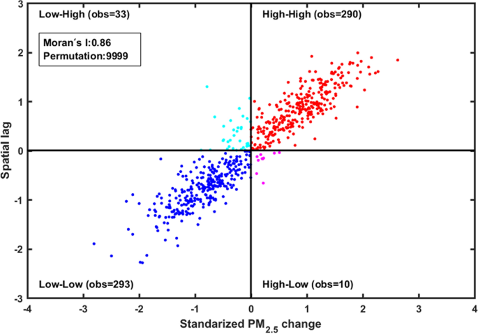
The computation of Moran’s I enables the identification of hot spots and cold spots. The hot spots are high-high clusters where the increase in the PM2.5 level is higher than the surrounding areas, whereas cold spots are low-low clusters with the presence of low values in a low-value neighborhood. A Moran scatterplot, with x-axis as the original variable and y-axis as the spatially lagged variable, reflects the spatial association pattern. The slope of the linear fit to the scatter plot is an estimation of the global Moran's I72 (Fig. 2). The plot consists of four quadrants, each defining the relationship between an observation74. The upper right quadrant indicates hot spots and the lower left quadrant displays cold spots75.
Moran’s I scatterplot. Figure was produced by R 3.4.376.
Division based on population size
The last division was based on population size, which is a proven factor in changing per capita emissions in a wide selection of global cities, even outperformed land urbanization rate77,78,79. We used the 2014 urban population to classify the cities into four groups based on United Nations definitions80: (1) large agglomerations with a total population larger than 1 million; (2) mid-sized cities, 500,000–1 million; (3) small cities, 250,000–500,000, and (4) very small cities, 100,000–250,000.
Panel data analysis
The panel data analysis is an analytical method that deals with observations from multiple entities over multiple periods. Its capacity in analyzing the characteristics and changes from both the time-series and cross-section dimensions of data surpasses conventional models that purely focus on one dimension81,82. The estimation equation for the panel data model in this study is given as:
where the subscript \(i\) and \(t\) refer to city and year respectively. \(\upbeta _{{0}}\) is the intercept parameter and \(\upbeta _{{1}} - { }\upbeta _{{{18}}}\) are the estimates of slope coefficients. \(\varepsilon \) is the random error. All variables are transformed into natural logarithms.
Two methods can be used to obtain model estimates, separately fixed effects estimator and random effects estimator. The fixed effects estimator assumes that each subject has its specific characteristics due to inherent individual characteristic effects in the error term, thereby allowing differences to be intercepted between subjects. The random effects estimator assumes that the individual characteristic effect changes stochastically, and the differences in subjects are not fixed in time and are independent between subjects. To choose the right estimator, we run both models for each group of cities based on the Hausman specification test83. The null hypothesis is that random effects model yields consistent and efficient estimates84: \({H}_{0}{:}\,E\left({\varepsilon }_{i}|{X}_{it}\right)=0\). If the null hypothesis is rejected, the fixed effects model will be selected for further inferences. Once the better estimator was determined for each model, one optimal panel data model was fit to each city group of one division type. In total, six, four, and eight runs were conducted for socioeconomic, spatial autocorrelation, and population division separately and three, two, and four panel data models were finally selected.
Results
Spatial patterns of PM2.5 level changes
During the period from 2000 to 2014, the annual mean PM2.5 concentration of all cities increases from 27.78 to 42.34 µg/m3, both of which exceed the World Health Organization recommended annual mean standard (10 µg/m3). It is worth noting that the PM2.5 level in the year 2014 also exceeds China’s air quality Class 2 standard (35 µg/m3) that applies to non-national park places, including urban and industrial areas. The standard deviation of annual mean PM2.5 values for all cities increases from 12.34 to 16.71 µg/m3, which shows a higher variability of inter-urban PM2.5 pollution after a decadal period. The least and most heavily polluted cities in China are Delingha, Qinghai (3.01 µg/m3) and Jizhou, Hubei (64.15 µg/m3) in 2000 and Hami, Xinjiang (6.86 µg/m3) and Baoding, Hubei (86.72 µg/m3) in 2014.
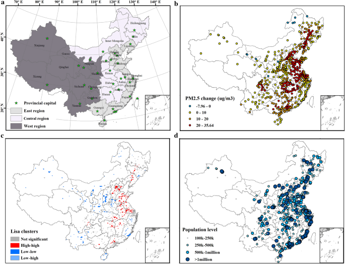
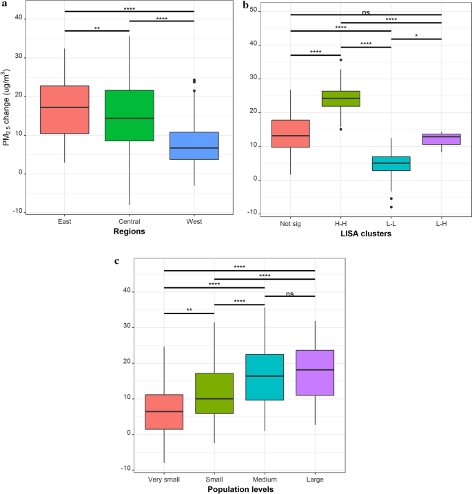
Spatially, the changes in PM2.5 levels exhibit heterogeneous patterns across cities (Fig. 3b). According to the socioeconomic level division (Fig. 3a), the Eastern, Central, and Western region experienced a 38.6, 35.3, and 25.5 µg/m3 increase in annual PM2.5 mean, separately, and the difference among regions is significant according to the analysis of variance (ANOVA) results (Fig. 4a). When stratified by spatial autocorrelation relationship (Fig. 3c), the differences in PM2.5 changes among the spatial clusters are even more dramatic. The average PM2.5 increase in cities belonging to the high-high cluster is approximately 25 µg/m3, as compared to 5 µg/m3 in the low-low clusters (Fig. 4b). Finally, cities at four different population levels have significant differences in the changes of PM2.5 concentration (Fig. 3d), except for the mid-sized cities and large city agglomeration (Fig. 4c).
(a) Division of cities in China by socioeconomic development level and the locations of provincial capitals; (b) Changes in annual mean PM2.5 concentrations between the year 2000 and 2014; (c) LISA cluster maps for PM2.5 changes at the city level; High-high indicates a statistically significant cluster of high PM2.5 level changes over the study period. Low-low indicates a cluster of low PM2.5 inter-annual variation; No high-low cluster is reported; Low–high represents cities with high PM2.5 inter-annual variation surrounded by cities with low variation; (d) Population level by cities in the year 2014. Maps were produced by ArcGIS 10.7.185.
Boxplots of PM2.5 concentration changes between 2000 and 2014 for city groups that are formed according to (a) socioeconomic development level division, (b) LISA clusters, and (c) population level. Asterisk marks represent the p value of ANOVA significant test between the corresponding pair of groups. Note ns not significant; *p value < 0.05; **p value < 0.01; ***p value < 0.001; H–H high-high cluster, L–H low–high cluster, L–L denotes low–low cluster.
The effects of urban forms on PM2.5 changes
The Hausman specification test for fixed versus random effects yields a p value less than 0.05, suggesting that the fixed effects model has better performance. We fit one panel data model to each city group and built nine models in total. All models are statistically significant at the p < 0.05 level and have moderate to high predictive power with the R2 values ranging from 0.63 to 0.95, which implies that 63–95% of the variation in the PM2.5 concentration changes can be explained by the explanatory variables (Table 2).
The urban form—PM2.5 relationships differ distinctly in Eastern, Central, and Western China. All models reach high R2 values. Model for Eastern China (refer to hereafter as Eastern model) achieves the highest R2 (0.90), and the model for the Western China (refer to hereafter as Western model) reaches the lowest R2 (0.83). The shape metrics FRAC and CONTIG are correlated with PM2.5 changes in the Eastern model, whereas the area metrics AREA demonstrates a positive effect in the Western model. In contrast to the significant associations between shape, area metrics and PM2.5 level changes in both Eastern and Western models, no such association was detected in the Central model. Nonetheless, two aggregation metrics, LSI and AI, play positive roles in determining the PM2.5 trends in the Central model.
For models built upon the LISA clusters, the H–H model (R2 = 0.95) reaches a higher fitting degree than the L–L model (R2 = 0.63). The estimated coefficients vary substantially. In the H–H model, the coefficient of CONTIG is positive, which indicates that an increase in CONTIG would increase PM2.5 pollution. In contrast, no shape metrics but one area metrics AREA is significant in the L–L model.
The results of the regression models built for cities at different population levels exhibit a distinct pattern. No urban form metrics was identified to have a significant relationship with the PM2.5 level changes in groups of very small and mid-sized cities. For small size cities, the aggregation metrics COHESION was positively associated whereas AI was negatively related. For mid-sized cities and large agglomerations, CONTIG is the only significant variable that is positively related to PM2.5 level changes.
Discussion
Urban form is an effective measure of long-term PM2.5 trends
All panel data models are statistically significant regardless of the data group they are built on, suggesting that the associations between urban form and ambient PM2.5 level changes are discernible at all city levels. Importantly, these relationships are found to hold when controlling for population size and gross domestic product, implying that the urban landscape patterns have effects on long-term PM2.5 trends that are independent of regional economic performance. These findings echo with the local, regional, and global evidence of urban form effect on various air pollution types5,14,21,22,24,39,78 .
Although all models demonstrate moderate to high predictive power, the way how different urban form metrics respond to the dependent variable varies. Of all the metrics tested, shape metrics, especially CONTIG has the strongest effect on PM2.5 trends in cities belonging to the high-high cluster, Eastern, and large urban agglomerations. All those regions have a strong economy and higher population density86. In the group of cities that are moderately developed, such as the Central region, as well as small- and mid-sized cities, aggregation metrics play a dominant negative role in PM2.5 level changes. In contrast, in the least developed cities belonging to the low-low cluster regions and Western China, the metrics describing size and number of urban patches are the strongest predictors. AREA and NP are positively related whereas TA is negatively associated.
The impacts of urban form metrics on air quality vary by urbanization degree
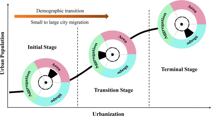
Based on the above observations, how urban form affects within-city PM2.5 level changes may differ over the urbanization stages. We conceptually summarized the pattern in Fig. 5: area metrics have the most substantial influence on air pollution changes at the early urban development stage, and aggregation metrics emerge at the transition stage, whereas shape metrics affect the air quality trends at the terminal stage. The relationship between urban form and air pollution has rarely been explored with such a wide range of city selections. Most prior studies were focused on large urban agglomeration areas, and thus their conclusions are not representative towards small cities at the early or transition stage of urbanization.
Not surprisingly, the area metrics, which describe spatial grain of the landscape, exert a significant effect on PM2.5 level changes in small-sized cities. This could be explained by the unusual urbanization speed of small-sized cities in the Chinese context. Their thriving mostly benefited from the urbanization policy in the 1980s, which emphasized industrialization of rural, small- and mid-sized cities87. With the large rural-to-urban migration and growing public interest in investing real estate market, a side effect is that the massive housing construction that sometimes exceeds market demand. Residential activities decline in newly built areas of smaller cities in China, leading to what are known as ghost cities88. Although ghost cities do not exist for all cities, high rate of unoccupied dwellings is commonly seen in cities under the prefectural level. This partly explained the negative impacts of TA on PM2.5 level changes, as an expanded while unoccupied or non-industrialized urban zones may lower the average PM2.5 concentration within the city boundary, but it doesn’t necessarily mean that the air quality got improved in the city cores.
Aggregation metrics at the landscape scale is often referred to as landscape texture that quantifies the tendency of patch types to be spatially aggregated; i.e., broadly speaking, aggregated or “contagious” distributions. This group of metrics is most effective in capturing the PM2.5 trends in mid-sized cities (population range 25–50 k) and Central China, where the urbanization process is still undergoing. The three significant variables that reflect the spatial property of dispersion, separately landscape shape index, patch cohesion index, and aggregation index, consistently indicate that more aggregated landscape results in a higher degree of PM2.5 level changes. Theoretically, the more compact urban form typically leads to less auto dependence and heavier reliance on the usage of public transit and walking, which contributes to air pollution mitigation89. This phenomenon has also been observed in China, as the vehicle-use intensity (kilometers traveled per vehicle per year, VKT) has been declining over recent years90. However, VKT only represents the travel intensity of one car and does not reflect the total distance traveled that cumulatively contribute to the local pollution. It should be noted that the private light-duty vehicle ownership in China has increased exponentially and is forecast to reach 23–42 million by 2050, with the share of new-growth purchases representing 16–28%90. In this case, considering the increased total distance traveled, the less dispersed urban form can exert negative effects on air quality by concentrating vehicle pollution emissions in a limited space.
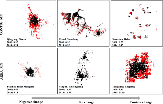
Finally, urban contiguity, observed as the most effective shape metric in indicating PM2.5 level changes, provides an assessment of spatial connectedness across all urban patches. Urban contiguity is found to have a positive effect on the long-term PM2.5 pollution changes in large cities. Urban contiguity reflects to which degree the urban landscape is fragmented. Large contiguous patches result in large CONTIG_MN values. Among the 626 cities, only 11% of cities experience negative changes in urban contiguity. For example, Qingyang, Gansu is one of the cities-featuring leapfrogs and scattered development separated by vacant land that may later be filled in as the development continues (Fig. 6). Most Chinese cities experienced increased urban contiguity, with less fragmented and compacted landscape. A typical example is Shenzhou, Hebei, where CONTIG_MN rose from 0.27 to 0.45 within the 14 years. Although the 13 counties in Shenzhou are very far scattered from each other, each county is growing intensively internally rather than sprawling further outside. And its urban layout is thus more compact (Fig. 6). The positive association revealed in this study contradicts a global study indicating that cities with highly contiguous built-up areas have lower NO2 pollution22. We noticed that the principal emission sources of NO2 differ from that of PM2.5. NO2 is primarily emitted with the combustion of fossil fuels (e.g., industrial processes and power generation)6, whereas road traffic attributes more to PM2.5 emissions. Highly connected urban form is likely to cause traffic congestion and trap pollution inside the street canyon, which accumulates higher PM2.5 concentration. Computer simulation results also indicate that more compact cities improve urban air quality but are under the premise that mixed land use should be presented18. With more connected impervious surfaces, it is merely impossible to expect increasing urban green spaces. If compact urban development does not contribute to a rising proportion of green areas, then such a development does not help mitigating air pollution41.
Six cities illustrating negative to positive changes in CONTIG_MN and AREA_MN. Pixels in black show the urban areas in the year 2000 and pixels in red are the expanded urban areas from the year 2000 to 2014. Figure was produced by ArcGIS 10.7.185.
Conclusions
This study explores the regional land-use patterns and air quality in a country with an extraordinarily heterogeneous urbanization pattern. Our study is the first of its kind in investigating such a wide range selection of cities ranging from small-sized ones to large metropolitan areas spanning a long time frame, to gain a comprehensive insight into the varying effects of urban form on air quality trends. And the primary insight yielded from this study is the validation of the hypothesis that the determinants of PM2.5 level trends are not the same for cities at various developmental levels or in different geographic regions. Certain measures of urban form are robust predictors of air quality trends for a certain group of cities. Therefore, any planning strategy aimed at reducing air pollution should consider its current development status and based upon which, design its future plan. To this end, it is also important to emphasize the main shortcoming of this analysis, which is generally centered around the selection of control variables. This is largely constrained by the available information from the City Statistical Yearbook. It will be beneficial to further polish this study by including other important controlling factors, such as vehicle possession.
References
Lim, C. C. et al. Association between long-term exposure to ambient air pollution and diabetes mortality in the US. Environ. Res. 165, 330–336 (2018).
Yang, J. & Zhang, B. Air pollution and healthcare expenditure: implication for the benefit of air pollution control in China. Environ. Int. 120, 443–455 (2018).
Bell, J. N. B., Power, S. A., Jarraud, N., Agrawal, M. & Davies, C. The effects of air pollution on urban ecosystems and agriculture. Int. J. Sust. Dev. World 18(3), 226–235 (2011).
Matus, K. et al. Health damages from air pollution in China. Glob. Environ. Change 22(1), 55–66 (2012).
Bereitschaft, B. & Debbage, K. Urban form, air pollution, and CO2 emissions in large US metropolitan areas. Prof Geogr. 65(4), 612–635 (2013).
Bozkurt, Z., Üzmez, Ö. Ö., Döğeroğlu, T., Artun, G. & Gaga, E. O. Atmospheric concentrations of SO2, NO2, ozone and VOCs in Düzce, Turkey using passive air samplers: sources, spatial and seasonal variations and health risk estimation. Atmos. Pollut. Res. 9(6), 1146–1156 (2018).
Fang, C., Liu, H., Li, G., Sun, D. & Miao, Z. Estimating the impact of urbanization on air quality in China using spatial regression models. Sustainability 7(11), 15570–15592 (2015).
Khaniabadi, Y. O. et al. Mortality and morbidity due to ambient air pollution in Iran. Clin. Epidemiol. Glob. Health 7(2), 222–227 (2019).
Health Effects Institute. State of Global Air 2019. Special Report (Health Effects Institute, Boston, 2019). ISSN 2578-6873.
O’Meara, M. & Peterson, J. A. Reinventing Cities for People and the Planet (Worldwatch Institute, Washington, 1999).
World Health Organization. Ambient Air Pollution: A Global Assessment of Exposure and Burden of Disease. ISBN: 9789241511353 (2016).
Liu, C. et al. Ambient particulate air pollution and daily mortality in 652 cities. N. Engl. J. Med. 381(8), 705–715 (2019).
Anderson, W. P., Kanaroglou, P. S. & Miller, E. J. Urban form, energy and the environment: a review of issues, evidence and policy. Urban Stud. 33(1), 7–35 (1996).
Hart, R., Liang, L. & Dong, P. L. Monitoring, mapping, and modeling spatial–temporal patterns of PM2.5 for improved understanding of air pollution dynamics using portable sensing technologies. Int. J. Environ. Res. Public Health. 17(14), 4914 (2020).
Environmental Protection Agency. Our Built and Natural Environments: A Technical Review of the Interactions Between Land Use, Transportation and Environmental Quality (2nd edn.). Report 231K13001 (Environmental Protection Agency, Washington, 2013).
Chen, M., Zhang, H., Liu, W. & Zhang, W. The global pattern of urbanization and economic growth: evidence from the last three decades. PLoS ONE 9(8), e103799 (2014).
Wang, S., Liu, X., Zhou, C., Hu, J. & Ou, J. Examining the impacts of socioeconomic factors, urban form, and transportation networks on CO2 emissions in China’s megacities. Appl. Energy. 185, 189–200 (2017).
Borrego, C. et al. How urban structure can affect city sustainability from an air quality perspective. Environ. Model. Softw. 21(4), 461–467 (2006).
Bart, I. Urban sprawl and climate change: a statistical exploration of cause and effect, with policy options for the EU. Land Use Policy 27(2), 283–292 (2010).
Feng, H., Zou, B. & Tang, Y. M. Scale- and region-dependence in landscape-PM2.5 correlation: implications for urban planning. Remote Sens. 9, 918. https://doi.org/10.3390/rs9090918 (2017).
Rodríguez, M. C., Dupont-Courtade, L. & Oueslati, W. Air pollution and urban structure linkages: evidence from European cities. Renew. Sustain. Energy Rev. 53, 1–9 (2016).
Bechle, M. J., Millet, D. B. & Marshall, J. D. Effects of income and urban form on urban NO2: global evidence from satellites. Environ. Sci. Technol. 45(11), 4914–4919 (2011).
Martins, H., Miranda, A. & Borrego, C. Urban structure and air quality. In Air Pollution-A Comprehensive Perspective (2012).
Stone, B. Jr. Urban sprawl and air quality in large US cities. J. Environ. Manag. 86(4), 688–698 (2008).
Breheny, M. Densities and sustainable cities: the UK experience. In Cities for the new millennium, 39–51 (2001).
Glaeser, E. L. & Kahn, M. E. Sprawl and urban growth. In Handbook of regional and urban economics, vol. 4, 2481–2527 (Elsevier, Amsterdam, 2004).
Manins, P. C. et al. The impact of urban development on air quality and energy use. Clean Air 18, 21 (1998).
Troy, P. N. Environmental stress and urban policy. The compact city: a sustainable urban form, 200–211 (1996).
Gaigné, C., Riou, S. & Thisse, J. F. Are compact cities environmentally friendly?. J. Urban Econ. 72(2–3), 123–136 (2012).
Wood, C. Air pollution control by land use planning techniques: a British-American review. Int. J. Environ. Stud. 35(4), 233–243 (1990).
Zhou, B., Rybski, D. & Kropp, J. P. The role of city size and urban form in the surface urban heat island. Sci. Rep. 7(1), 4791 (2017).
Sarrat, C., Lemonsu, A., Masson, V. & Guedalia, D. Impact of urban heat island on regional atmospheric pollution. Atmos. Environ. 40(10), 1743–1758 (2006).
Liu, Y., Wu, J., Yu, D. & Ma, Q. The relationship between urban form and air pollution depends on seasonality and city size. Environ. Sci. Pollut. Res. 25(16), 15554–15567 (2018).
Cavalcante, R. M. et al. Influence of urbanization on air quality based on the occurrence of particle-associated polycyclic aromatic hydrocarbons in a tropical semiarid area (Fortaleza-CE, Brazil). Air Qual. Atmos. Health. 10(4), 437–445 (2017).
Han, L., Zhou, W. & Li, W. Fine particulate (PM2.5) dynamics during rapid urbanization in Beijing, 1973–2013. Sci. Rep. 6, 23604 (2016).
Tuo, Y., Li, X. & Wang, J. Negative effects of Beijing’s air pollution caused by urbanization on residents’ health. In 2nd International Conference on Science and Social Research (ICSSR 2013), 732–735 (Atlantis Press, 2013).
Zhou, C. S., Li, S. J. & Wang, S. J. Examining the impacts of urban form on air pollution in developing countries: a case study of China’s megacities. Int. J. Environ. Res. Public Health. 15(8), 1565 (2018).
Cariolet, J. M., Colombert, M., Vuillet, M. & Diab, Y. Assessing the resilience of urban areas to traffic-related air pollution: application in Greater Paris. Sci. Total Environ. 615, 588–596 (2018).
She, Q. et al. Air quality and its response to satellite-derived urban form in the Yangtze River Delta, China. Ecol. Indic. 75, 297–306 (2017).
Yang, D. et al. Global distribution and evolvement of urbanization and PM2.5 (1998–2015). Atmos. Environ. 182, 171–178 (2018).
Cho, H. S. & Choi, M. Effects of compact urban development on air pollution: empirical evidence from Korea. Sustainability 6(9), 5968–5982 (2014).
Li, C., Wang, Z., Li, B., Peng, Z. R. & Fu, Q. Investigating the relationship between air pollution variation and urban form. Build. Environ. 147, 559–568 (2019).
Montgomery, M. R. The urban transformation of the developing world. Science 319(5864), 761–764 (2008).
United Nations. World Urbanization Prospects: The 2009 Revision (United Nations Publication, New York, 2010).
Jiang, L. & O’Neill, B. C. Global urbanization projections for the shared socioeconomic pathways. Glob. Environ. Change 42, 193–199 (2017).
Martine, G., McGranahan, G., Montgomery, M. & Fernandez-Castilla, R. The New Global Frontier: Urbanization, Poverty and Environment in the 21st Century (Earthscan, London, 2008).
Gong, P., Li, X. C. & Zhang, W. 40-Year (1978–2017) human settlement changes in China reflected by impervious surfaces from satellite remote sensing. Sci. Bull. 64(11), 756–763 (2019).
Center for International Earth Science Information Network—CIESIN—Columbia University, C. I.-C.-I.. Global Rural–Urban Mapping Project, Version 1 (GRUMPv1): Urban Extent Polygons, Revision 01. Palisades, NY: NASA Socioeconomic Data and Applications Center (SEDAC) (2017). https://doi.org/10.7927/H4Z31WKF. Accessed 10 April 2020.
Balk, D. L. et al. Determining global population distribution: methods, applications and data. Adv Parasit. 62, 119–156. https://doi.org/10.1016/S0065-308X(05)62004-0 (2006).
Chinese Academy of Surveying and Mapping—CASM China in Time and Space—CITAS—University of Washington, a. C.-C. (1996). China Dimensions Data Collection: China Administrative Regions GIS Data: 1:1M, County Level, 1 July 1990. Palisades, NY: NASA Socioeconomic Data and Applications Center (SEDAC). https://doi.org/10.7927/H4GT5K3V. Accessed 10 April 2020.
Ma, L. J. Urban administrative restructuring, changing scale relations and local economic development in China. Polit. Geogr. 24(4), 477–497 (2005).
Van Donkelaar, A. et al. Global estimates of fine particulate matter using a combined geophysical-statistical method with information from satellites, models, and monitors. Environ. Sci. Technol. 50(7), 3762–3772 (2016).
Gong, P. et al. Annual maps of global artificial impervious area (GAIA) between 1985 and 2018. Remote Sens. Environ 236, 111510 (2020).
Li, X. C., Gong, P. & Liang, L. A 30-year (1984–2013) record of annual urban dynamics of Beijing City derived from Landsat data. Remote Sens. Environ. 166, 78–90 (2015).
Li, X. C. & Gong, P. An, “exclusion-inclusion” framework for extracting human settlements in rapidly developing regions of China from Landsat images. Remote Sens. Environ. 186, 286–296 (2016).
National Bureau of Statistics 2000–2014. China City Statistical Yearbook (China Statistics Press). ISBN: 978-7-5037-6387-8
Lai, A. C., Thatcher, T. L. & Nazaroff, W. W. Inhalation transfer factors for air pollution health risk assessment. J. Air Waste Manag. Assoc. 50(9), 1688–1699 (2000).
Luo, Y. et al. Relationship between air pollutants and economic development of the provincial capital cities in China during the past decade. PLoS ONE 9(8), e104013 (2014).
Hart, R., Liang, L. & Dong, P. Monitoring, mapping, and modeling spatial–temporal patterns of PM2.5 for improved understanding of air pollution dynamics using portable sensing technologies. Int. J. Environ. Res. Public Health 17(14), 4914 (2020).
Wang, X. & Zhang, R. Effects of atmospheric circulations on the interannual variation in PM2.5 concentrations over the Beijing–Tianjin–Hebei region in 2013–2018. Atmos. Chem. Phys. 20(13), 7667–7682 (2020).
Xu, Y. et al. Impact of meteorological conditions on PM2.5 pollution in China during winter. Atmosphere 9(11), 429 (2018).
Hernandez, G., Berry, T.A., Wallis, S. & Poyner, D. Temperature and humidity effects on particulate matter concentrations in a sub-tropical climate during winter. In Proceedings of the International Conference of the Environment, Chemistry and Biology (ICECB 2017), Queensland, Australia, 20–22 November 2017; Juan, L., Ed.; IRCSIT Press: Singapore, 2017.
Zhang, Y. Dynamic effect analysis of meteorological conditions on air pollution: a case study from Beijing. Sci. Total. Environ. 684, 178–185 (2019).
National Earth System Science Data Center. National Science & Technology Infrastructure of China. https://www.geodata.cn. Accessed 6 Oct 2020.
Bhatta, B., Saraswati, S. & Bandyopadhyay, D. Urban sprawl measurement from remote sensing data. Appl. Geogr. 30(4), 731–740 (2010).
Dietzel, C., Oguz, H., Hemphill, J. J., Clarke, K. C. & Gazulis, N. Diffusion and coalescence of the Houston Metropolitan Area: evidence supporting a new urban theory. Environ. Plan. B Plan. Des. 32(2), 231–246 (2005).
Li, S., Zhou, C., Wang, S. & Hu, J. Dose urban landscape pattern affect CO2 emission efficiency? Empirical evidence from megacities in China. J. Clean. Prod. 203, 164–178 (2018).
Gyenizse, P., Bognár, Z., Czigány, S. & Elekes, T. Landscape shape index, as a potencial indicator of urban development in Hungary. Acta Geogr. Debrecina Landsc. Environ. 8(2), 78–88 (2014).
Rutledge, D. T. Landscape indices as measures of the effects of fragmentation: can pattern reflect process? DOC Science Internal Series. ISBN 0-478-22380-3 (2003).
Mcgarigal, K. & Marks, B. J. Spatial pattern analysis program for quantifying landscape structure. Gen. Tech. Rep. PNW-GTR-351. US Department of Agriculture, Forest Service, Pacific Northwest Research Station, 1–122 (1995).
Chan, C. K. & Yao, X. Air pollution in mega cities in China. Atmos. Environ. 42(1), 1–42 (2008).
Anselin, L. The Moran Scatterplot as an ESDA Tool to Assess Local Instability in Spatial Association. In Spatial Analytical Perspectives on Gis in Environmental and Socio-Economic Sciences (eds Fischer, M. et al.) 111–125 (Taylor; Francis, London, 1996).
Zou, B., Peng, F., Wan, N., Mamady, K. & Wilson, G. J. Spatial cluster detection of air pollution exposure inequities across the United States. PLoS ONE 9(3), e91917 (2014).
Bone, C., Wulder, M. A., White, J. C., Robertson, C. & Nelson, T. A. A GIS-based risk rating of forest insect outbreaks using aerial overview surveys and the local Moran’s I statistic. Appl. Geogr. 40, 161–170 (2013).
Anselin, L., Syabri, I. & Kho, Y. GeoDa: an introduction to spatial data analysis. Geogr. Anal. 38, 5–22 (2006).
R Core Team. R A Language and Environment for Statistical Computing (R Foundation for Statistical Computing, Vienna, 2013).
Cole, M. A. & Neumayer, E. Examining the impact of demographic factors on air pollution. Popul. Environ. 26(1), 5–21 (2004).
Liu, Y., Arp, H. P. H., Song, X. & Song, Y. Research on the relationship between urban form and urban smog in China. Environ. Plan. B Urban Anal. City Sci. 44(2), 328–342 (2017).
York, R., Rosa, E. A. & Dietz, T. STIRPAT, IPAT and ImPACT: analytic tools for unpacking the driving forces of environmental impacts. Ecol. Econ. 46(3), 351–365 (2003).
United Nations, Department of Economic and Social Affairs Population Division 2011: the 2010 Revision (United Nations Publications, New York, 2011)
Ahn, S. C. & Schmidt, P. Efficient estimation of models for dynamic panel data. J. Econ. 68(1), 5–27 (1995).
Du, L., Wei, C. & Cai, S. Economic development and carbon dioxide emissions in China: provincial panel data analysis. China Econ. Rev. 23(2), 371–384 (2012).
Hausman, J. A. Specification tests in econometrics. Econ. J. Econ. Soc. 46(6), 1251–1271 (1978).
Greene, W. H. Econometric Analysis (Pearson Education India, New Delhi, 2003).
ArcGIS GIS 10.7.1. (Environmental Systems Research Institute, Inc., Redlands, 2010).
Lao, X., Shen, T. & Gu, H. Prospect on China’s urban system by 2020: evidence from the prediction based on internal migration network. Sustainability 10(3), 654 (2018).
Henderson, J.V., Logan, J.R. & Choi, S. Growth of China's medium-size cities. Brookings-Wharton Papers on Urban Affairs, 263–303 (2005).
Lu, H., Zhang, C., Liu, G., Ye, X. & Miao, C. Mapping China’s ghost cities through the combination of nighttime satellite data and daytime satellite data. Remote Sens. 10(7), 1037 (2018).
Frank, L. D. et al. Many pathways from land use to health: associations between neighborhood walkability and active transportation, body mass index, and air quality. JAPA. 72(1), 75–87 (2006).
Huo, H. & Wang, M. Modeling future vehicle sales and stock in China. Energy Policy 43, 17–29 (2012).
Acknowledgements
Lu Liang received intramural research funding support from the UNT Office of Research and Innovation. Peng Gong is partially supported by the National Research Program of the Ministry of Science and Technology of the People’s Republic of China (2016YFA0600104), and donations from Delos Living LLC and the Cyrus Tang Foundation to Tsinghua University.
Author information
Authors and Affiliations
Contributions
L.L. and P.G. wrote the main manuscript text. All authors reviewed the manuscript.
Corresponding author
Ethics declarations
Competing interests
The authors declare no competing interests.
Additional information
Publisher's note
Springer Nature remains neutral with regard to jurisdictional claims in published maps and institutional affiliations.
Rights and permissions
Open Access This article is licensed under a Creative Commons Attribution 4.0 International License, which permits use, sharing, adaptation, distribution and reproduction in any medium or format, as long as you give appropriate credit to the original author(s) and the source, provide a link to the Creative Commons licence, and indicate if changes were made. The images or other third party material in this article are included in the article's Creative Commons licence, unless indicated otherwise in a credit line to the material. If material is not included in the article's Creative Commons licence and your intended use is not permitted by statutory regulation or exceeds the permitted use, you will need to obtain permission directly from the copyright holder. To view a copy of this licence, visit http://creativecommons.org/licenses/by/4.0/.
About this article
Cite this article
Liang, L., Gong, P. Urban and air pollution: a multi-city study of long-term effects of urban landscape patterns on air quality trends. Sci Rep 10, 18618 (2020). https://doi.org/10.1038/s41598-020-74524-9
Received:
Accepted:
Published:
DOI: https://doi.org/10.1038/s41598-020-74524-9
This article is cited by
-
Spatial–temporal distribution patterns and influencing factors analysis of comorbidity prevalence of chronic diseases among middle-aged and elderly people in China: focusing on exposure to ambient fine particulate matter (PM2.5)
BMC Public Health (2024)
-
The association between ambient air pollution exposure and connective tissue sarcoma risk: a nested case–control study using a nationwide population-based database
Environmental Science and Pollution Research (2024)
-
Systematic review of ecological research in Philippine cities: assessing the present status and charting future directions
Discover Environment (2024)
-
The evolution of atmospheric particulate matter in an urban landscape since the Industrial Revolution
Scientific Reports (2023)
-
Simulation of particle resuspension by wind in an urban system
Environmental Fluid Mechanics (2023)
Comments
By submitting a comment you agree to abide by our Terms and Community Guidelines. If you find something abusive or that does not comply with our terms or guidelines please flag it as inappropriate.

