
Abstract
We present a multiphase model for solid tumor initiation and progression focusing on the properties of cancer stem cells (CSC). CSCs are a small and singular cell sub-population having outstanding capacities: high proliferation rate, self-renewal and extreme therapy resistance. Our model takes all these factors into account under a recent perspective: the possibility of phenotype switching of differentiated cancer cells (DC) to the stem cell state, mediated by chemical activators. This plasticity of cancerous cells complicates the complete eradication of CSCs and the tumor suppression. The model in itself requires a sophisticated treatment of population dynamics driven by chemical factors. We analytically demonstrate that the rather important number of parameters, inherent to any biological complexity, is reduced to three pivotal quantities.Three fixed points guide the dynamics, and two of them may lead to an optimistic issue, predicting either a control of the cancerous cell population or a complete eradication. The space environment, critical for the tumor outcome, is introduced via a density formalism. Disordered patterns are obtained inside a stable growing contour driven by the CSC. Somewhat surprisingly, despite the patterning instability, the contour maintains its circular shape but ceases to grow for a typical size independently of segregation patterns or obstacles located inside.
Introduction
Discrete1,2,3 and continuous4 models have been proposed recently to study solid tumor progression within the cancer stem cells (CSCs) hypothesis. According to this concept5, CSCs are a small subpopulation within the tumor that are the main cause for its progression. These cells have high proliferation rates, self-renewal and quasi-immortality capacities6,7. Consequently, they are very difficult to detect and to eradicate. The cancer stem cell hypothesis has been matter of strong debates during the last forty years8. Nevertheless it explains several biological evidences such as the relapse of tumor post-surgery and treatments9 or the ability to generate tumors in xenotransplantation10. Nowadays, surface biomarkers, in charge of identification and detection of these cells, are more and more evaluated for different classes of cancer which allows new therapeutics in clinical11 but also experimental measurements of their physical properties12.
The CSC model13 enters into a more general class, usually referred as hierarchical models where cancer cells originate from a precursor which divides either symmetrically giving two identical CSCs or two DCs (differentiated cancer cells) or asymmetrically (one CSC and one DC). In these models, only the complete extinction of the CSC population eradicates the tumor. The stochastic model, instead, considers the possibility that every cell can be a tumor-initiating one and so the best eradication strategy becomes a more complex issue. Our work lies between both concepts: indeed, as stated by Plaks et al.14, this distinction is often a false dichotomy because of the phenotype plasticity of cancerous cells15 which allows to recover the stem traits by dedifferentiation. The same feature also occurs with healthy differentiated cells which are known to gain a stem state under traumatic conditions, but not only, and this plasticity process seems much more common than previously believed8. Within these ideas, we propose a rather simple dynamical tumor initiation model in the continuous limit, for a mixed population, composed of 3 subpopulations: cancer stem cells (CSCs), differentiated cancer cells (DCs) and all other cells that a tumor harbors such as quiescent, dead or immune cells. Each cell population, represented by its density, enters a nonlinear dynamical system based on proliferation rates controlled by chemical pathways and physical interactions. We demonstrate that the dynamics is governed by the existence and stability of 3 fixed points showing the possibility of full tumor extinction, but also of over-shooting dynamics after a period of remission or relapse of the tumor post surgery.These features, observed in practice, are not commonly recovered in cancer growth modeling16,17 when biological parameters are fixed.
According to activator and inhibitor concentrations which control the growth rate or the phenotypic changes6,8, a phase-diagram is presented, which shows the exchange of stability as a function of a very limited number (3) of pivotal parameters. Focusing on the conditions for final extinction by a proper selection of the parameters is indeed a crucial goal for efficient therapeutic strategies9, giving hope to bypass the cell plasticity.
We also aim to determine the spatial cellular repartition during tumor progression. From a physical viewpoint, we provide a methodology for the study of ternary mixtures which have been poorly investigated, especially for free boundary growing domains18,19,20. Involving cell-cell interaction and solid-fluid friction, the mechanics is based on variational analysis which leads to a set of coupled partial-differential equations (PDE). The simulations tackle space inhomogeneity, possible obstacles, applied exterior stresses and the emergence of different tumors in the same neighborhood, then mimicking more closely the tumoral micro-environement and giving a most realistic picture of growing tumors in patients. In addition, the basic concepts are not limited to cancer research and may also apply to other ecologic21 or societal models22,23, where a colony expands thanks to a very active and aggressive sub-population.
The Theoretical Model
We restrict ourselves to 3 kinds of cells with the same mass density: cancer stem cells (CSC), differentiated cancer cells (DC) and all other cells (C) or constituents such as interstitial fluids. In a closed environment, the concentrations S, for CSC, D for DC and C for inert constituents satisfy the relation S + D + C = 1. We simplify the proliferation process of the CSCs, eliminating intermediate progenitors24,25. The main characteristic of stem-ness is the fact of symmetric or asymmetric divisions leading to clones into the hierarchy that we describe in terms of probabilities (see Fig. (1a)). CSCs divide either symmetrically, giving two CSCs with probability p1 or two DCs with probability p2, or asymmetrically with probability 1 − p1 − p2. Then the probability to gain 2 CSCs per division reads 2p = (1 + p1 − p2) while it becomes 2(1 − p) = 1 − p1 + p2 for DC cells, see Fig. (1a). The mitosis of CSC is simultaneously controlled chemically by an activator a and an inhibitor i.a is produced by the CSCs (via the Wnt-β pathways26), and i is produced by the DCs, aiming to prevent the uncontrolled growth of S. Consequently, the probability 2p will increase with the activator concentration a saturating for large a values while the inhibitor i will decrease the p value as D increases. However, when S becomes exceptionally low, (falling below a tiny S0 value), mitosis alone is not sufficient for re-population of the CSC community. There is strong experimental evidence that a feedback exists, originating from phenotypic changes of DC cells switching back to the CSC state. Also called cancer cell plasticity, this process is governed by an activator m which can be a network of miniRNA27 for example. Surprisingly, in a sorted population with only DCs, where this process happens, it does not lead to an over-shoot of the CSC population, so the effect is weak but relatively sharp around the S0 value.

(a) Schematic presentation of the model corresponding to the set of equations Eq. (1) (b) Phase diagram for existence and stability of fixed points in the plane of dimensionless parameters d,q0. Regions are separated by d = q0 and by d = ψα/β. The range γ/α > m0 has been selected. Stable fixed points are represented by a square, saddle fixed points by a speech bubble. In the plastic region, d < q0, the value of the parameters are intimately related, m2 being always close to m0 indicating an easy phenotypic switching and so plasticity. Close to \({{\mathscr{ {\mathcal F} }}}_{2}\), tumor cells are then in the highest plastic state. In the following, Table 2 classifies all the fixed points in each region of the phase diagram.
In summary, the dynamics of cell population and of the chemicals is governed by a set of 4 coupled differential equations with smooth variations4, except for the activator m1 which varies sharply around the value S ~ S0. All these assumptions explain the following set of equations:
where p(D, a) and q(m) satisfy:
At this stage, the spatial variation is ignored and the time unit t0 has been chosen as the inverse of the mitotic rate of the CSCs. CSCs are considered as immortal, as opposed to DCs and to the chemicals a or m, so no death rate is added for S. According to the second equation of Eq. (1), the DC proliferation and death are included in the single parameter d. Excessive growth of D leads to the disappearance of CSCs, the so-called Allee effect, demonstrated by Konstorum et al.4 and to an optimistic issue for tumor elimination. Unfortunately, as CSCs tend to disappear, the de-differentiation (or plasticity) occurs from DC to CSC, controlled by m as shown in Fig. (1). Then, the Allee effect may be compromised by the re-population of CSCs, and ultimately of DCs, which happens for m greater than a typical value m0. To ensure a sharp variation of q(m), the parameter σ which enters the last equation of Eq. (2) is a tiny quantity and a real feedback DCs versus CSCs is possible if γ/α > m0. In practice, in vivo or in vitro, the population of CSCs is always a tiny fraction of the entire tumor population (few per cents). When S is below this tiny value, the activator m starts to grow as q(m), leading to an increase of S. Notice that the time-scale for de-differentiation q0, Eq. (2), has to be compared to the symmetric mitotic rate but the issue of this dynamical system depends on the comparison of q0 with d (the time death rate of DCs) and with α (time elimination rate of both chemicals a and m which are chosen equal for simplification). As in4, the dynamics of a results from the positive competition between the activator itself, the CSC’s population S and the spontaneous degradation rate α. To conclude, in our model, the selected biological ingredients of the CSCs hypothesis leads to a dynamical system of population of fourth order with a minimal set of 8 parameters, two of them having small values as S0 and σ. As demonstrated in the next section and suggested by the phase diagram in Fig.(1b), only 3 parameters really control the full dynamics and the tumor progression.
Dynamics: Fixed Points, Stability, Basin of Attraction
Existence of fixed points
The strategy of population dynamics consists in the search of fixed points, achieved by cancelling all time derivatives in Eq. (1). Followed by stability analysis, this part does not present any difficulty and details can be found in the Appendix (A). Here we only focus on the main results. Fixed points represent static and homogeneous solutions of the physical system, which is assumed to be spatially infinite. Defined by the 4 concentrations: \({ {\mathcal F} }_{i}\) = {Si, Di, ai, mi}, they share in common 2 relationships:
so only Si and ai must be determined since Si determines both Di and mi. A calculation with ai = 0, so p = 0 leads to 2 fixed points: S1 = 0 or \({S}_{2}=-\,{S}_{0}\,\log (\frac{\alpha }{\gamma }{m}_{2})\). The first fixed point accepts arbitrary m1 value, \({ {\mathcal F} }_{1}\) = {0, 0, 0, m1} and corresponds to the full tumor extinction. For the second choice, m2 satisfies:
according to Eq. (1). In other words, this second fixed point only exists under two conditions: first, there is no self-proliferation of the DCs and second, cancerous cell plasticity occurs. The first condition then implies that the D cells are in an homeostatic state. In practice, both S and D must remain smaller than 1 just like their sum, but more importantly S and D must remain positive leading to a new inequality m2 < γ/α. Then, the existence of the second fixed point imposes the following inequalities of parameters: 0 < d < q0 and m2 < γ/α.
Considering now ai ≠ 0, the third equation of Eq. (1) gives S3 = α(1 + a3)/(βa3), so \({m}_{3}=\gamma /a{e}^{-{S}_{3}/{S}_{0}}\) and finally D3 = S3/d, see Eqs (16, 25). However, the first equation must be verified leading to (2p(D3,a3) − 1)d + q = 0 so p ~ 1/2, for small S0 and σ. An algebraic equation of second order for a3 gives a positive solution if ψ < d(β/α) (see Appendix C). Then the existence of this third fixed point requires an efficient but not too strong retro-action originating from the DCs.
A summary of these conclusions can be found in the phase-diagram in Fig. (1b) which shows that 2 fixed points always exist, \({ {\mathcal F} }_{1}\) and \({ {\mathcal F} }_{3}\), contrary to \({ {\mathcal F} }_{2}\) which only exists if 0 < d < q0. Independently of the parameter restrictions, these fixed points are potentially relevant for tumor growth if they are stable with a finite basin of attraction. This is the reason why we consider now the dynamics of small perturbations, described by the linearization of the right-hand-side of Eq. (1).
Stability of the fixed points
At linear order, rewritten in matrix form, it reads:
where (δ\({ {\mathcal F} }_{i}\))T is the transpose of δ\({ {\mathcal F} }_{i}\) and J(\({ {\mathcal F} }_{i}\)) is the Jacobian calculated for each fixed point (see the Appendix A). The stability is governed by the sign of the real part λR of the eigenvalues λi of the Jacobian matrix: it is stable if all λR values are negative (locally an attractor), unstable if all eigenvalues are positive (a repeller), and saddle in the general case. Each fixed point must be treated separately with technical aspects explained in the Appendix B,C and the stability results are functions of the model parameters which are summarized here:
-
(a)
\({ {\mathcal F} }_{1}\) = (0, 0, 0, m1), which leads to the full tumor extinction, is stable and attractive if d > q(m1). If the feedback of DCs versus CSCs is not too strong in comparison with the death rate of D. Since q(m1) < q0, the stability condition for \({ {\mathcal F} }_{1}\) is simply d > q0 which means d above the first bisector in the phase-diagram Fig. (1b). In Figure (2a), the monotonous decays of both S(t) and D(t) from an initial set parameters inside the basin of attraction of \({ {\mathcal F} }_{1}\) are outlined.
Figure 2 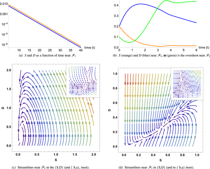
(a,b) Cancer cell S and D evolution near fixed points \({ {\mathcal F} }_{1}\) and \({ {\mathcal F} }_{2}\). (c,d) Streamlines determine the direction of attraction or repulsion near the fixed points for the tumor cells and the chemicals. Due to the high dimensionality of the system we project the dynamics along two directions, while keeping the other two constant. In (c,d) A complex pair of eigenvalues with negative real part determines a spiral point in the {S, D} plane. Differently, the other two eigenvalues are real and negative, making the point \({ {\mathcal F} }_{2}\) globally stable (c). (c,d) arrows determine the direction of attraction or repulsion near the fixed points for the tumor cells and the chemicals and the colors, increasing from purple to red, are the relative norms of the vector fields. Due to the high dimensionality of the system, we project the dynamics along two directions, while keeping the other two constant.
-
(b)
\({ {\mathcal F} }_{2}\) = (S2, S2/d, 0, m2) means a low population for both CSCs and DCs. It is always stable when it exists (d < q0) below the first bisector in a phase-diagram Fig.(1b). In Figure (2b,c), from an initial set of parameters inside the basin of attraction of \({ {\mathcal F} }_{2}\), the streamlines and the dynamics of both S(t) and D(t) are presented. The concentrations exhibit an over-shooting behavior before reaching the equilibrium values (see Fig. (2b)) and that the streamlines are disordered in Fig. (2c).
-
(c)
The dynamics of \({ {\mathcal F} }_{3}\) is more complex and requires appropriate approximations. Assuming ψ < dβ/α, it is at least a saddle point, possibly an unstable point, see Fig. (2d) where it is a saddle fixed point.

To conclude, among all parameters of the model, only d and q0 play a pivotal role. It exists always a stable fixed point with low cancerous cell concentration: either \({ {\mathcal F} }_{1}\) or \({ {\mathcal F} }_{2}\). When \({ {\mathcal F} }_{2}\) appears, for d < q0, \({ {\mathcal F} }_{1}\) becomes unstable. When \({ {\mathcal F} }_{3}\) exists, it is never stable. For a clinical perspective, to reach either \({ {\mathcal F} }_{1}\) or \({ {\mathcal F} }_{2}\) takes a great importance. However when the feedback and plasticity of DCs is too weak compared to their death rate, the emergence of \({ {\mathcal F} }_{3}\) may compromise these optimistic solutions. One can wonder if the scenario depicted here is maintained when the feedback parameter q0 becomes a time-dependent variable, q0 = q0(t) or if some chemical values as a or m become stochastic. This may occur for multiple reasons, the main coming from the genetic of cancerous cells, mutation after mutation. Another reason may be environmental factors, changing in the chemicals activity as drug for example. In the Appendix, D, we perform numerical simulations of the dynamical model, Eq. (1), with a time-dependent q0(t) and we give preliminary results on stochastic effects.
Strategy for tumor regression
The previous analysis shows the dramatic role of two quantities: d and q(m) representing respectively the DCs proliferation rate (d < 0) or the DCs death rate (d > 0) and q(m) the DCs dedifferentiation rate. A parameter d < 0 (by absorption of nutrients, for example) induces an exponential growth in both populations of CSCs and DCs. Even for d > 0, (by senescence or death via drug treatments), it may not be sufficient even if the death rate d is stronger than the plasticity represented by q(m). In other words, if d > q(m) holds, it will not imply automatically a regression in all cases due to the vicinity of the third repulsive fixed point \({ {\mathcal F} }_{3}\).
The ideal case would be to remain in the blue region of the diagram, (Fig.(1b)), where there exists a unique stable fixed point \({ {\mathcal F} }_{1}\), insisting that, in this case, q(m1) < d < ψα/β. The most obvious strategy will consist in reducing q(m) as much as possible so that the first inequality becomes easier to reach. Since m1 = γ/α (see Eq. (3)) if m1 < m0, then q(m1) ~ 0, the first inequality is checked and there is hope to reach complete extinction of the tumor by eradicating both CSCs and DCs. Notice that, it requires also the second inequality to be verified. In this case, one should control the degradation rate α of the activators which plays a crucial role. Increasing α will be the best way to lead the tumor to extinction. Moreover, controlling the aggressiveness of the self-renewal activator via the parameter β as well as the inhibitory feedback of the DCs via ψ (Eq. (2) makes this situation more likely to occur (see Fig. (6a,b) in the Appendix D.1). The inset of Fig. (2c) representing the (S, a) subspace at fixed value d = 0 shows the small size of the basin of attraction, meaning that even at low levels of S and a, the tumor cannot undergo full tumor regression and differentiated cells may be produced again. Considering now m0s and m1 fixed, varying σ will not affect too much q(m1) since σ only controls the smoothness of the function q(m).
Suppose now that m1 > m0, then q(m1) ~ q0. The worst scenario occurs when d < q0 because the stable attractive fixed point will be the second one \({ {\mathcal F} }_{2}\). What we would really like to do is to decrease as much as possible the value of S2 and D2, concentrations of CSCs and DCs respectively. But, S2 is of order S0, D2 is of order S0/d. It will be difficult to decrease these cancerous populations since they are dependent on biological parameters that we cannot control. Estimation of the time scale for proliferation of CSCs depends on the cancer origin. In27, the rate of cell division is about 1.8 month−1, and estimation of the de-differentiation factor is of order 0.6 per month. In pancreatic xenograft tumors, the rate of CSCs division is about 10 month−1 and the level of activator, normalized to 1 for healthy tissue, is about 4 for unsorted cancer cells, becoming 46 for selected and sorted CSCs28. Introducing these to Eq. (1), we derive α/β ~ 0.2 and d ~ 0.3. In Table 1, experimental results have been collected. Even if the biological literature on the subject is very rich these last years, it is unfortunate that not so much quantitative physical or chemical informations are available.Finally in29, the inhibitor i has been identified explaining why patients with high level in lung tumor have a better prognosis.
Thus, the best strategy seems to target the chemical activators rather than the cancerous cells. Indeed, the presence of the cancer stem cells effectively drives the tumor, even in the optimistic case where we hopefully kill all the cancer cells, still CSCs will differentiate again and start a new cycle making the treatment very unlikely to succeed when the chemical activators are not controlled, (compare the two figures Fig. (6a,b) in the Appendix D.1 which shows how the basin of attraction of a stable point can be reduced). In medical centers nowadays, this strategy is commonly employed post-surgery to avoid the relapse of a new tumor at the same place of the primary one which has been withdrawn. Long-time drug administration over years aims at suppressing these activators.
The analysis of this model is very rich. However, it assumes an infinite geometry and the results must be confronted to the spatial structure of the host tissue. It is the reason why we now focus on the spatial evolution of a tumor seed, with initial conditions in the vicinity of the fixed point \({ {\mathcal F} }_{2}\).
Spatio-Temporal Dynamics of Tumor Growth
Population dynamics modeling gives only a first overview of tumoro-genesis, far from the real complexity driven by cell-cell interactions, friction with other cells or with the stroma and physical perturbations due to obstacles, that are always present in the host organ. In addition, in many cancers, the primary tumor, once detected, is not unique and may be accompanied by smaller satellites. So the spatial component cannot be ignored as well. As shown in30, for inhomogeneous in vivo tumor, the density of each constituent varies locally, and the spatio-temporal behavior is completely different from the one predicted by a dynamical system. It is even worse when a spinodal decomposition19 occurs leading to a a phase separation of Cahn-Hilliard type inside the tumor31,32. Furthemore, the possible existence of niches, area of localization of S cells, introduces a new complexity that we will not consider here. They do not seem to be present in every tumor and are believed to be dependent on the patient’s age, as reported by Ferraro and Lo Clesio33. Besides, most of the physical characteristics of the cancerous niche such as their localization and density in the host tissue have not been reported even in recent review papers as6,8,26 which focus mostly on biological pathways.
Given the diversity of situations for human beings, a unique model cannot exist and the same strategy is adopted here for CSCs and DCs. Our dynamical system must be completed by adding the standard advective term \(\nabla \cdot ({\varphi }_{i}{\overrightarrow{v}}_{i})\) in the left-hand-side of Eq. (1), ϕi representing either S, D or a, m. It reads:
For the chemicals, a or m, we restrict on diffusion and \({\overrightarrow{v}}_{i}=-\,{D}_{i}\nabla {\varphi }_{i}/{\varphi }_{i}\). The average velocity of cells \({\overrightarrow{v}}_{i}\) will be derived from the Rayleighian variation, counter-part of the Lagrangian for highly dissipative systems34,35, taking into account the constraints of the Galilean Invariance: \(\nabla (S{\overrightarrow{v}}_{S}+D{\overrightarrow{v}}_{D}+C{\overrightarrow{v}}_{C})=0\) in addition to S + D + C = 1 (see the Appendix E). Then, cell velocities result from proliferation and mechanical forces. CSCs being much less numerous and more individualist with a propensity to escape and make metastasis, we neglect their energy of cohesion. Thus, the free energy of the cell mixing E is dominated by the DCs36, and we only consider the mixing energy of DCs:
Ω(t) defining the tumor domain in expansion, χ only depends on the density D, the last term being a penalty for sharp transitions19,35,37. At the border, the micro-environment acts as a hydrostatic pressure. Little is known on cell-cell interaction of CSCs with DCs, but the mixing energy is scaled by the square of cell densities giving a net advantage to the DCs, responsible for the tumor cohesion. The cellular elasticity is discarded: recent AFM38,39 or nano-indentation experiments40 indicate that cancerous cells are less stiff than their healthy counterparts by 70% or 80%, due to an alteration and regression of their cytoskeleton. Since inertia is negligible, viscous dissipation controls the dynamics which is determined by a variational process acting on the Rayleighian (for technical details see Appendix E). Taking into account the principle of extremum of this quantity with the incompressibility constraint gives the following velocities for \({\overrightarrow{v}}_{D}\) and \({\overrightarrow{v}}_{S}\):
From Eq. (8), we can define the cell-cell adhesion in units of τ which gives a length unit l0 as the square root of the cell-cell adhesion multiplied by t0, the time unit, so hereafter all quantities will be dimensionless. For simplicity, we do not change the notations. Different options can be made for χD but must respect physical objectives such as balance of the stresses at the tumor border, itself defined by a border density Db although this condition assumes no density gradient at the border. In addition, at low densities, χ is close to zero, being negative and strongly increases for growing density above Db. A standard choice is the Cahn-Hilliard potential,(see Appendix E) but here, by reason of numerical convergence the potential introduced by Byrne and Preziosi41,42 has been preferred. Its derivative reads:
αD, DB and Λ being positive constants. Db is smaller than 1.
Heterogeneity under tumor growth
Adopting the same strategy as before, we extend the stability analysis of each dynamically stable fixed point, \({ {\mathcal F} }_{1}\) and \({ {\mathcal F} }_{2}\), to spatially periodic perturbations such that each cell or chemical density becomes ϕ(x, t) = ϕhomo + (δϕ)eλtcos(kx). Each Jacobian (Eqs (5) and (41)) is then dependent on k2 and the characteristic polynomial \(P(\lambda )=\mathop{\sum }\limits_{j=0}^{3}\,{\lambda }^{j}{C}_{j}({k}^{2})\) which fixes the eigenvalues can be found in the Appendix F. Static and periodic patterns are found for λ = dλ/dk = 0 which imposes that C0 = dC0(k)/dk = 0 as well.
At linear order, advection does not play any role for \({ {\mathcal F} }_{1}\) since S1 = D1 = 0, and the diffusion of chemicals being stabilizing, this fixed point remains stable leading to a homogeneous tumor. As predicted by the linear stability analysis explained in Appendix F and shown in Fig. (3a,b), there exist patterns for \({ {\mathcal F} }_{2}\). The selected wavenumber of the spatial pattern is found in the neighborhood of \({k}_{c}^{2}\sim -\,1/(2{e}^{2})\chi ^{\prime\prime} \), so for D2 ~ 0.44 according to our choice given by Eq. (9). One can observe that low values of D2 (i.e. below 0.44) make segregation more likely to occur. Patterns in a square are shown in Fig. (3c,d) and in Fig. (4) in a growing tumor. Notice that in the vicinity of the selected D2 values, the numerical patterns exhibit either unstable labyrinths or dots. Dots may represent the nests (clinical vocabulary) observed in many tumors. Assuming the soft tissue to be homogeneous, the tumoral seed develops with a phase segregation inside, both for CSCs and DCs, (see Fig.(4a,b)). Surprisingly, despite the interior patterning, the contour remains rather well defined with no contour instability except when obstacles are introduced. With a small density of random obstacles, (see Fig. (4c,d)) the interface is tortuous but in (e) it surprisingly recovers regularity at a high density. CSCs are more located at border except the case of low level of obstacles. This CSCs concentration at the border of tumors is also observed in mice after injection of human CSCS43. The fact that CSC have a higher density at the border also indicates that they are good candidate for metastasis. Finally, in Fig. (5), 3 seeds are introduced to mimic more closely the clinical reality. Details on the numerics are given in Section (Methods), however one must mention that modelling of growing tumors is numerically much more challenging when not achieved in a square with periodic boundary conditions.

Cell repartition study in the vicinity of fixed points \({ {\mathcal F} }_{2}\) in the domain of dynamical stability (see Fig. (1b)). In (a,b), results of the linear stability analysis with variation of the wave number k revealed by C0. In (a), the dynamical parameters are: \({ {\mathcal F} }_{2}\) = (0.2D2, D2, 0,0.2), with α = 1, Da = Dm = 1 and B = −5. in (b) the same parameter but with B = −20 (see Eq. (16) of the Appendix C). The Byrne-Preziozi potential41,42 is selected with the following values αD = 2, m = 1, Db = 0.6 and εD = 0.1 in Eq. (9). Phase separation of tumor cell CSC or DC with the surrounding tissue. In (c): Labyrinth-like pattern for {d, α} = {0.2, 1} and consequentially {D2, S2} ~ {0.23, 0.045}. (d): Honeycomb-like pattern for {d,α} = {0.15,0.8} and consequentially {D2, S2} ~ {0.4, 0.06}.

Growing tumors in different tissues and chemical conditions: (a,b) in a homogeneous tissue, represented by a standard grid in the simulations, (c,d) in a tissue with 2% of randomly distributed obstacles, (e) in a tissue with 5% of randomly distributed obstacles. (f) Activator a density in a medium with high density of obstacles. All patterns are scaled by the length unit l0, square root of the ratio between the cell-cell adhesion density and the friction coefficient times the time unit so l0 = (t0χ/τ)1/2.

Population of cancer stem cells (a) and differentiated cancer cells (b) in growing tumors starting from three initial equidistant and separated seeds. Even for primary tumors (non metastatic), it is not rare that several tumors can be found in the same neighborhood.
Discussion and Conclusion
In this paper, we presented, analyzed and simulated a simple multiphase model for tumor initiation driven by CSC cells. We focused both on the differentiation process of cancer stem cells and on the de-differentiation of differentiated cancer cells within the tumor. We analyzed the effect of chemical activators responsible for these processes and the possible therapeutic strategies for tumor extinction. Our conclusion is that, in this situation, the most effective strategies are the ones that target chemical activators rather than cells themselves, due to a vicious feedback loop between CSCs and DCs. New therapeutics emerge in this direction29,44,45. With numerical simulations, we understood how modifications of the environment, in which the tumor expands, can abruptly change its long time behavior. In the future, a clear understanding of the mechanical and physical properties of CSCs can improve the model, especially when considering adhesion energy, elastic deformation and cell-cell interaction41,46. In this spirit, a more complicated multiphase model can be constructed, taking into account immune cells, the host cells and their interaction with tumor cells. Because of a lack of information, the existence of niches is dogged here: they may be at the origin of localized sources of D cells inside the tumor and would require separation between mobile and static DC populations. Our model can be extended to other cellular cell types which can be reprogrammed in cancer initiated cells47 or in cancer stem cells after responses to therapeutics48. From the theoretical viewpoint, we have treated here an ecological model where the competition between species depends on a singular tiny sub-population. It will apply probably to other communities than the cancerous cells, opening future directions in nonlinear physics.
Methods
The system corresponding to Fig. (6) was numerically solved with the XMDS2 software package49. We used an adaptive Runge-Kutta of fourth-fifth order with a tolerance 10−5. All spatial operators were evaluated via spectral methods. The simulations were performed on a (400 × 400) grid with a space discretization of dx = 10−1 and with periodic boundary conditions for Fig. (3) which shows the emergence of different patterns with respect to the fixed point values \({ {\mathcal F} }_{2}\). The most relevant parameters d and α were varied, keeping fixed in the following the ensemble {η, ψ, q0, m0, σ, β, γ} = {1, 1, 1, 0.5, 0.05, 1, 1} and {εD, εS, εC, Λ, Db, αD, Dm, Da} = {0.1, 0, 0, 2, 0.6, 2, 1, 1}. In Fig. (3c) different choices for chemical degradation rates and cell death result in labyrinth-like patterns for both S and D. In Fig. (3d), upon increasing the value \({ {\mathcal F} }_{2}\), a honeycomb-like pattern emerges. The origin of the different patterns may be due to the highest value of D2 which increases the effective strength of the cell-cell DCs attraction given by Eq. (9). In Fig. (4) an initially localized concentration of CSCs and DCs grows in space and time. Numerical simulations were performed for different boxes and initial conditions. In Fig. (4) from a to f, S, D are initialized as a small and localized population with random perturbations around \({ {\mathcal F} }_{2}\). Similar initial conditions apply for the chemicals, but distributed on the entire grid. Concentration fields for both S,D are evaluated up to t = 30 - the time scale being in unit of differentiation of the CSCs - and plotted against each other. In Fig. (4a,b), CSCs and DCs expand in a homogeneous tissue. In particular, Fig. (4a) highlights the relevance of CSCs in this process. CSCs form a ring of higher concentration with respect to bulk values which effectively drives the tumor. In Fig. (4) from c to f, obstacles are introduced inside the box. Obstacles are tumor regions not accessible to tumor cells. In order to model them, simulations were performed on a grid with randomly distributed holes. Numerically, at each step of the iterative process, we cancel the cell density inside the holes corresponding to obstacles and then we integrate the following discretized equation \(\frac{\partial {\varphi }_{i}}{\partial t}=({\Gamma }_{{\varphi }_{i}}-{\nabla }_{i}\cdot {\varphi }_{i}{\overrightarrow{v}}_{{\varphi }_{i}}){O}_{i}\). Oi is a (1,0) binary variable, extracted from a Bernoulli distribution with a different mean: μ = 0.98 in Fig. (4c,d) and μ = 0.95 in Fig. (4e,f). In Fig. (4c,d) the tumor grows in a tortuous fashion, breaking the cylindrical symmetry. This effect is two-sided: first, the addition of obstacles breaks the circular ring and second, the values of \({ {\mathcal F} }_{2}\) are the same as the honeycomb pattern, giving rise to a strong effective attraction between cells. In Fig. (4e), despite a higher number of holes in the grid, the only relevant effect to the tumor growth is the breakdown of the circular ring of CSCs. The size and form of the tumor are qualitatively unaffected.

(a) Basin of attraction for tumor extinction in case of controlled chemical feedback ({β, α, η, ψ} = {3, 1, 1, 1}). (b) The basin of attraction of tumor extinction shrinks as the chemicals are less controlled, making the extinction less likely to occur ({β, α, η, ψ} = {5, 0.2, 2, 2}). In (a), an initial concentration of CSCs will undergo regression and so DCs for every meaningful value of chemicals concentrations. In (b), the shrinkage of the basin of attraction for tumour regression may lead to an invasive colony of cancer cells, even in case of a small initial concentration.
Our dynamical model presents 3 fixed points, 2 of them are of special interest since they concern a low concentration of cancerous cells. Their stability and basin of attraction have a crucial importance for treatments: they can induce the complete disappearance of the cancer cells. Each fixed point Fi is defined by 4 concentrations values \({ {\mathcal F} }_{i}\) = (Si, Di, ai, mi) which satisfy the dynamical system Eq. (1), without time dependence. The notation ϕj is used for either S, D, a or m. Following a very classical strategy of dynamical systems50,51, each concentration ϕ is perturbed according to \({\tilde{\varphi }}_{j}={\varphi }_{j}+{\delta }_{j}{e}^{{\lambda }_{i}t}\) where δj is a small quantity and λj the growth rate of the perturbation. The stability is entirely governed by the Jacobians of our system, Eq. (10), having coefficient matrix given by ∂Γk/∂ϕj where Γk has been introduced to represent dϕk/dt. Being local, the stability analysis must be achieved for each fixed point, independently of the others.

In (a) Relaxation to the steady state value of differentiated cell population D near the stable point \({ {\mathcal F} }_{1}\) with Runge-Kutta algorithm. Initial concentration {S(0), D(0), m(0), a(0)} = {0.1, 0.1, 1.0, 1.0}. With such initial parameters, the system is in the basin of attraction of the first fixed point, so of tumor extinction. The S concentration (not represented here) follows the same lines. Time is in the unit of the mitotic rate of S cells, see Section (Methods). In (b)CSCs and DCs (orange and blue respectively) oscillate with a delay with respect to the oscillating activity q0(t) (light red curve). DCs need CSCs to differentiate, causing a delay in their productions. Likewise, CSCs need DCs to dedifferentiate. Other values of ω and ε have been tested, without obtaining any substantial difference but a time scale.
References
La Porta, C. A. M., Zapperi, S. & Sethna, J. P. Senescent Cells in Growing Tumors: Population Dynamics and Cancer Stem Cells. Domany E, ed. PLoS Computational Biology 8(1), e1002316 (2012).
Enderling, H., Hlatky, L. & Hahnfeldt, P. Cancer stem cells: a minor cancer subpopulation that redefines global cancer features. Front. Oncol., https://doi.org/10.3389/fonc.2013.00076 (2013).
La Porta, C. A. M. & Zapperi, S. The Physics of Cancer. Cambridge University Press (2017).
Konstorum, A., Hillen, T. & Lowengrub, J. Feedback Regulation in a Cancer Stem Cell Model can Cause an Allee effect. Bull. Math. Biological. 78(4), 754–785 (2016).
Driessens, G., Beck, C., Caauwe, A., Simons, B. D. & Blanpain, C. Defining the mode of tumour growth by clonal analysis. Nature 488, 527–530 (2012).
Soteriou, D. & Fuchs, Y. A matter of life and death: stem cell survival in tissue regeneration and tumor formation. Nature Review cancer 1–15 (2018).
Pattabiraman, D. R. & Weinberg, R. Tackling the cancer stem cells-what challenges do they pose? Nat. Rev. Drug. Discov. 13(7), 497–512 (2014).
Battle, E. & Clevers, H. Cancer stem cells revisited. Nat. Med. 23(10), 1124–1134 (2017).
Chang, J. C. Cancer stem cells: Role in tumor growth, recurrence, metastasis, and treatment resistance”. Medicine (Baltimore) Sep; 95(1,Suppl 1), S20–5, https://doi.org/10.1097/MD.0000000000004766 (2016).
Munthe, S. et al. Migrating glioma cells express stem cell markers and give rise to new tumors upon xenograftin. Journal of neuro-oncology 130, 53–62 (2016).
Krause, M., Dubrovska, A. D., Linge, A. & Baumann, M. Cancer stem cells: Radioresistance, prediction of radiotherapy outcome and specific targets for combined treatments. Advanced Drug Delivery Reviews 109, 63–73 (2017).
Polizzi, S. et al. A minimal rupture cascade model for living cell plasticity. New J. Phys. 20, 053057 (2018).
Nassar, D. & Blanpain, C. Cancer Stem Cells: Basic Concepts and Therapeutic Implications. Annu.Rev. Pathol. Mech. Dis. 11, 47–76 (2016).
Plaks, V., Kong, N. & Werb, Z. The Cancer Stem Cell Niche: How Essential is the Niche in Regulating Stemness of Tumor Cells. Cell stem cell. 8(10), 755–768 (2008).
Cabrera, M. C., Hollingsworth, R. E. & Hurt, E. M. Cancer stem cell plasticity and tumor hierarchy. World J Stem Cells 7, 27–36 (2015).
Loh, J. K. et al. Arrested growth and spontaneous tumor regression of partially resected low-grade cerebellar astrocytomas in children. Nerv Syst 29, 2051–2055 (2013).
Kasahara, T. et al. Spontaneous Slowing and Regressing of Tumor Growth in Childhood/Adolescent Papillary Thyroid Carcinomas Suggested by the Postoperative Thyroglobulin-Doubling Time. Journal of Thyroid Research, Article ID 6470251, https://doi.org/10.1155/2018/6470251 (2018).
Ben Amar, M. Tumour growth modeling: physical insights to skin cancer. Mathematical Oncology, D’Onofrio, A. & Gandolfi, A. Editors. Springer (2014).
Bazant, M. Thermodynamic stability of driven open systems and control of phase separation by electro-autocatalysis. Faraday Discussions 199, 423–463 (2017).
Hoshino, T. et al. Pattern formation of skin cancers: Effects of cancer proliferation and hydrodynamic interactions. Phys. Rev. E 99(032416), 1–13 (2019).
Fernandez-Oto, C., Tzuk, O. & Meron, E. Front Instabilities Can Reverse Desertification. Phys. Rev. Lett. 122, 048101–05 (2019).
Bertozzi, A. L., Johnson, S. D. & Ward, M. J. Mathematical modelling of crime and security Special Issue of EJAM. European Journal of Applied Mathematics 27(3), 311–316 (2016).
Marshak, C. Z., Rombach, M. P., Bertozzi, A. L. & D’Orsogna, M. R. Growth and containment of a hierarchical criminal network. Phys. Rev. E 93(1–14), 022308 (2016).
Reya, T., Morrison, S. J., Clarke, M. F. & Weissman, I. L. Stem cells, cancer, and cancer stem cells. Nature 414, 105–111 (2001).
Shang, Z. et al. Isolation of cancer progenitor cells from cancer stem cells in gastric cancer. Mol Med Rep. 15(6), 3637–3643 (2017).
Visvader, J. E. & Lindeman, G. J. Cancer stem cells in solid tumors: accumulating evidence and unresolved questions. Nat Rev Cancer 16(3), 225–238 (2015).
Sellerio, A. L. et al. Overshoot during phenotypic switching of cancer cell populations. Scientific Reports 515464 (2015).
Li, C. et al. Identification of Pancreatic Cancer Stem Cells. Cancer Res. 7(3), 1030–37 (2007).
Liu, T., Wu, X., Chen, T., Luo, Z. & Hu, X. Downregulation of DNMT3A by miR-708-5p Inhibits Lung Cancer Stem Cell like Phenotypes through Repressing Wnt/β-catenin Signaling. Clin Cancer Res 24(7), 1748–1760 (2018).
Ben Amar, M., Chatelain, M. & Ciarletta, P. Contour instabilities in early tumor growth models. Phys. Rev. Lett. 106, 148101–4 (2011).
Cahn, J. W. & Hilliard, J. E. Free energy of a nonuniform system. I. Interfacial free energy. J. Chem. Phys 28, 258–267 (1958).
Chatelain, C., Balois, T., Ciarletta, P. & Ben Amar, M. Emergence of microstructural patterns in skin cancer: a phase separation analysis in a binary mixture. New Journ Physics 13, 115013–21 (2011).
Ferraro, F. & Lo Celso, C. Adult Stem cells and their niches. Adv.Exp. Med. Biot. 695, 155–168 (2010).
Doi, M. Onsager’s variational principle in soft matter. Journ. Phys.: Cond. Matt. 23(284118), 1–8 (2011).
Landau, L. D. & Ginzburg, V. Zh. Eksp. Teor. Fiz. 20, 1064 (1950).
Bocci, F. Levine, H., Onuchic & Jolly, M. K. Deciphering the dynamics of epithelial-mesenchymal transition and cancer stem cells in tumor progression. preprint.
van der Waals, J. The thermodynamik theory of capillarity under the hypothesis of a continuous variation of density. J. Stat. Phys. 20, 197–244 (1893).
Cross, S. E. et al. AFM-based analysis of human metastatic cancer cells. Nanotechnology 19(38), 384003 (2008).
Yallapu, M. M. et al. The Roles of Cellular Nanomechanics in Cancer. Med.Res.Rev. 35, 198–223 (2015).
Hayashi, K. & Iwata, M. Stiffness of cancer cells measured with an AFM indentation method. J Mech Behav Biomed Mater. 49, 105–11 (2015).
Preziosi, L. & Vitale, G. Chapter book: Mechanics of tumor growth:Multiphase models, adhesion and evolving configurations, Les Houches 2009: New trends in the Physics and Mechanics of Biological Systems, Oxford.
Byrne, H. & Preziosi, L. Modelling solid tumour growth using the theory of mixtures. Math. Med. Biol. 20, 341–366 (2003).
Prince, M. E. et al. Identification of a subpopulation of cells with cancer stem cell properties in head and neck squamous cell carcinoma. Proc. Nat. 104, 973–978 (2007).
Dashzeveg, N. K. et al. New Advances and Challenges of Targeting Cancer Stem Cells. Cancer Research 77(19), 5222–5227 (2017).
Jimeno, A. et al. A First-in-Human Phase I Study of the Anticancer Stem Cell Agent Ipafricept (OMP-54F28), a Decoy Receptor for Wnt Ligands, in Patients with Advanced Solid Tumors. Clin Cancer Res 23(24), 7490–7497 (2017).
Hale, J. S., Li, M. & Lathia, J. D. The malignant social network: cell-cell adhesion and communication in cancer stem cells. Cell Adh Migr. 6(4), 346–55 (2012).
Köhler, C. et al. Mouse Cutaneous Melanoma Induced by Mutant BRaf Arises from Expansion and Dedifferentiation of Mature Pigmented Melanocytes. Cell Stem Cell 21(5), 679–693 (2017).
Rambow, F. et al. Toward Minimal Residual Disease-Directed Therapy in Melanoma. Cell 174(4), 843–855 (2018).
Dennis, G. R., Hope, J. J. & Johnsson, M. T. XMDS2: Fast, scalable simulation of coupled stochastic partial differential equation. Computer Physics Communications 184(1), 201–208 (2013).
Strogatz, S.H. Nonlinear Dynamics and Chaos: With Applications to Physics, Biology, Chemistry, and Engineering,Westview Press (1994).
Meron, E. Nonlinear Physics of Ecosystems CRC Press Taylor & Francis Group (2015).
Hurwitz, A. On the conditions under which an equation has only roots with negative real parts Selected Papers on Mathematical Trends in Control Theory (R. Bellman and R. Kalaba Eds. New York: Dover),70 (1964).
Neubert, M. G. & Caswell, H. Ecology 78, 653 (1997).
Dufour, O. & Ben Amar, M. The role of stochasticity in the emergence of clonal patterns in tumor, ENS preprint (2019).
Jain, R. K. Transport of molecules in the tumor interstitium: a review. Cancer Res. 47, 3039–3051 (1987).
van Kemenade, P. M., Huyghe, J. M. & Douven, L. F. Triphasic FE modeling of skin water barrier. Transp. Porous Media 50, 93–109 (2003).
Swabb, E. A., Wei, J. & Gullino, P. M. Diffusion and convection in normal and neoplastic tissues. Cancer Res. 34, 2814–2822 (1974).
Acknowledgements
M.B.A. acknowledges the partial support from the Simons Foundation, the EPSRC Grant No. EP/K032208/1 and the Institut Universitaire de France. She would like to thank the Isaac Newton Institute of Mathematical Sciences, Cambridge, for support and hospitality during the program “Growth, Form and Self-Organization”. We would like to thank Giulia de Meijere for the critical reading of the manuscript.
Author information
Authors and Affiliations
Contributions
M.B.A. conceptualized and guided the project. F.O. and M.B.A. contributed to the theoretical modeling and wrote the manuscript. F.O. realized the simulations.
Corresponding author
Ethics declarations
Competing interests
The authors declare no competing interests.
Additional information
Publisher’s note Springer Nature remains neutral with regard to jurisdictional claims in published maps and institutional affiliations.
Appendix
A. Existence and stability of fixed points
The Jacobian matrix, calculated with the densities of each fixed point, is then:
B. Stability of the two first fixed points: \({ {\mathcal F} }_{1}\) and \({ {\mathcal F} }_{2}\)
This fixed point corresponds to complete eradication of the tumor. The Jacobian reads:
For this setting, the eigenvalues are:
with D2 = S2/d and S2 = −S0Log[(αm2)/γ]. After straightforward simplifications, the Jacobian for this fixed point is then:
One eigenvalue obviously being λ1 = −α, the three others are determined by solving the third order characteristic polynomial:
C. Existence and stability analysis of the fixed point \({ {\mathcal F} }_{3}\)
The existence of the third fixed point corresponds to q(m3) ~ 0 and p ~ 1/2, which allows to get an approximate value of a3 by solving p(a3, D3) = 1/2. It follows an algebraic second order equation for a3:
The treatment is more difficult for this fixed point if we do not make the appropriate approximations which lead to its condition of existence. Indeed, without approximation, from Eq. (10), the characteristic polynomial is expected to be of 4th order, then requiring a numerical treatment. Assuming that ψ0 is smaller than 1 but not too close to 1, we can consider that \({e}^{-{S}_{3}/{S}_{0}} \sim 0\), since S0 is a tiny quantity compared to \({S}_{3}=\frac{\alpha }{\beta }\frac{(1+{a}_{3})}{{a}_{3}}\). In addition, q(m3) ~ 0 and p ~ 1/2. This simplifies the Jacobian which reads:
which also indicates a saddle point. However, due to the number of independent parameters, the study of the roots of the characteristic polynomial of third order remains cumbersome. Indeed, the product of the 3 roots being positive indicates that at least one real eigenvalue is positive, suggesting that the third fixed point is always a saddle point, once it exists (ψ0 < 1), independently of all parameters.
D. Numerical investigation of the dynamical system
We select numerical values of parameters such that both \({ {\mathcal F} }_{1}\) and \({ {\mathcal F} }_{3}\) exist, the first one being stable but in the neighborhood of \({ {\mathcal F} }_{3}\) which is unstable. In this case and as shown in Fig. (1b), \({ {\mathcal F} }_{1}\) is the only attractive fixed point which gives the optimistic issue of the full tumor regression. However, \({ {\mathcal F} }_{3}\) can possibly prevent the cancer regression, even in such a favorable situation. We numerically focus on the set {α, β, d, ψ, η} = {1, 3, 2, 1, 1}, giving ψ0 = αψ/(dβ) = 1/6 which is smaller than 1 as required for the existence of \({ {\mathcal F} }_{3}\). Choosing {γ, m0, σ, S0, q0} = {1, 0.5, 0.05, 0.038, 1}, it is found \({ {\mathcal F} }_{1}\) = (0, 0, 0, 1), stable since d > q0 and from Eq. (19), we numerically deduce:
The value of σ is chosen to mimic conveniently a Heaviside function for q(m). The computed eigenvalues of the Jacobian from Eq. (10) corresponds perfectly to Eq. (23) which validates our approximated analysis of the stability of the third fixed point. It also proves that, for the determination of the eigenvalues which fixes the dynamics, the only pertinent parameters are {α, β, d, ψ, η} and that the precise values of {S0, σ, γ} have much less importance. For this particular choice, we have 3 directions of attraction, 2 being spirals and one being a repulsive direction, see Fig. (2d). As shown analytically, this is a saddle point. In Fig. (2a,b), the population of DC and CSC cells are given as a function of time in a log-scale where a time-scale relaxation can be estimated and compared to the smallest (in absolute value) growth rate predicted by Eq. (13), λ1(4) ~ −0.536, see Fig. (7a).
Here, \({ {\mathcal F} }_{1}\) will be repulsive, while \({ {\mathcal F} }_{2}\) will be attractive and \({ {\mathcal F} }_{3}\) is a saddle fixed point (c.f Fig.(1b)). The following parameters are selected: {α, β, d, ψ, η} = {0.5, 5, 0.2, 0.5, 1}, the other parameters being fixed as: {γ, m0, σ, S0, q0} = {1, 0.05, 0.038, 1}. For \({ {\mathcal F} }_{3}\) = {S3, D3, a3, m3} = {0.052, 0.26, 2.147, 0.51}. The eigenvalues for \({ {\mathcal F} }_{3}\) are calculated with Eq. (10) and gives the same results as Eq. (24). The situation looks similar to the previous case but the main and important difference relies on the existence of two repulsive fixed points, \({ {\mathcal F} }_{1}\) and \({ {\mathcal F} }_{3}\) (see Fig. (1b)). As shown in Fig. (2b), one striking feature is the overshoot of the dynamical variables induced by the feedback activator m. The tumor will not go under regression most of the time, although \({ {\mathcal F} }_{2}\) is an attractive fixed point, Fig. (2c). Moreover even when the system reaches a steady state, it can maintain a high level of differentiated cells if d is small. The tumor will not proliferate but may stabilize at dangerous levels, which is not an optimistic issue in practice.
We proceed by investigating the dynamics of the system numerically. We perform numerical simulations of Eq. (1) when q0(t) is an explicit time-dependent function. Of particular interest is the case where q0(t) oscillates around d, in the area of the bisector. In this regime, we would expect the system to exhibit an oscillatory behavior, due to the switching in the stability of the fixed points: \({ {\mathcal F} }_{1}\) <=> \({ {\mathcal F} }_{2}\). In particular, \({ {\mathcal F} }_{1}\) will change from a stable fixed point (tumor regression) to an unstable fixed point. The concentration of cells will then be pushed away from its decreasing value when at a particular time t1, q0(t1) > d and pushed back toward regression when q0(t2) < d. In Fig. (7), we show numerical results for q0 = d + f(t), f(t) being a periodic function with period T. Despite the symmetry around d, the system spending equal time in the different regions of the phase space, the tumor tends to go under regression at long times. Intuitively, the system relaxes to the different attractors in each regions (\({ {\mathcal F} }_{1}\) and \({ {\mathcal F} }_{2}\)) with a time scale governed by the slowest decaying mode. We compare the slowest decaying modes in the two extreme cases, q0(max) = d + fmax and q0(min) = d + fmin. In the first case, being q0(max) > d, the stable fixed point is \({ {\mathcal F} }_{2}\), with slowest decaying mode: λ = maxλi ~ −0.2 and associated time-scale \(\tau =\frac{1}{|\lambda |} \sim 5\). In the second case, q0(min) < d, the stable fixed point is \({ {\mathcal F} }_{1}\), with slowest decaying mode: λ = maxλi ~ −0.04 and associated time-scale \(\tau =\frac{1}{|\lambda |} \sim 25\). We would expect a faster relaxation toward \({ {\mathcal F} }_{2}\) than \({ {\mathcal F} }_{1}\), but this is not observed in Fig. (7). In particular, when the Jacobian matrices are not normal the instantaneous response -which determines the dynamic for a time varying q0(t)- is given by the eigenvalues of its hermitian part: HJ = (J + JT)/253. The hermitian matrix, HJ, has positive eigenvalues in both scenarios, making an analytical understanding of Fig. (7) challenging. Considering a and m as a stochastic variables, our preliminary study indicates that the noise stabilizes \({ {\mathcal F} }_{1}\) which seems to be selected rather than \({ {\mathcal F} }_{2}\) even in area where \({ {\mathcal F} }_{2}\) is stable without noise. This is especially verified above the bisector. Below the bisector, the answer is more complex but either \({ {\mathcal F} }_{1}\) or \({ {\mathcal F} }_{2}\) are selected. A more extensive study of stochasticity can be found in54. The results obtained for sinusoidal perturbations in the asymptotic may be due to the choice of initial data.
E. Spatio-dynamical equations deduced from the Rayleighian principle
The Rayleighian \( {\mathcal R} \) represents the energy variation per unit time for a system whose dynamics results only from dissipation, as for Stokes flow. When inertia is discarded, a variational principle of extremum of dissipation applies and the constraints acting on the system are included via Lagrange parameters Qi. It reads:
Let us first consider the dynamical equation inside the tumor. Considering an extremum of the Rayleighian with respect to \({\overrightarrow{v}}_{S}\), \({\overrightarrow{v}}_{D}\) and \({\overrightarrow{v}}_{C}\) gives the following 3 relationships:
First of all, it must be emphasized that our treatment is rather general and can be applied to any cell-cell interaction potential. In our simulations, no boundary conditions are required since our simulations correspond to an initial value problem and we do not take into account the exterior of the tumor assumed like a gel or a liquid. However, for completeness and future works, we briefly remind how they are determined from the variational process. They are helpful for selecting the densities Db and Sb which enter the free energies Eq. (37). In few cases, as for melanoma, the cancerous cell densities at border may be measured and the experimental values are chosen for Db and Sb. At the frontier, the interface velocity is the averaged velocity of the cancerous cells: \(\partial \dot{\Omega }(t)=(S{\overrightarrow{v}}_{S}+D{\overrightarrow{v}}_{D})/(S+D)\) if there is no phase separation. Indeed, it is possible that the mixing is fully inhomogeneous and that the phases split up from each other. Considering the terms which have been left by integration by part in the variation with respect to \({\overrightarrow{v}}_{D}\), we are faced with a contour integral:
Assuming that the border is the same for D and S cells (full mixing, no phase segregation) imposes \(\frac{\partial {\bar{\chi }}_{D}}{\partial D}=\frac{\partial {\bar{\chi }}_{S}}{\partial S}\). Choosing the Cahn-Hilliard free energy for χD and χS, (Eq. (37)), with D = Db and S = Sb leads to E = 0 and \(\frac{\partial {\bar{\chi }}_{D}}{\partial D}={a}_{D}{D}_{b}\) while \(\frac{\partial {\bar{\chi }}_{S}}{\partial S}={a}_{S}{S}_{b}\). So boundary conditions cannot be checked without the help of boundary layers of different thicknesses for both the S and D populations. A naive relationship will be found for the thicknesses of both boundary layers:
Having now the full spatio-dynamical equations, we can now investigate the stability analysis.
F. Stability analysis in the vicinity of dynamically stable fixed points
A spatial perturbation is added to any constituent of our system: ϕ(x, t) = ϕhomo + δϕ(t)cos(kx). The stability of the first fixed point will not change, for any wave-vector. For the second fixed point \({ {\mathcal F} }_{2}\), the Jacobian will be: J2k = J2 + k2/τδJ, J2 has yet been defined in Eq. (14) and δJ reads:
with all coefficients being dependent of k. This equation accepts 3 roots λ and a spatial static instability is obtained for the double condition C0 = −λ1λ2λ3 = 0 and dC0/dk = 0 which gives us the value of the threshold for instability and the wavelength at threshold. Due to the number of independent parameters, it is more convenient to fix the 3 parameters: α, B, d0 which partially define the initial fixed point \({ {\mathcal F} }_{2}\) up to the value of D2, so all the curves C0(k) will start at the same value and will differ because of D2. A representation of a spinodal decomposition can be found in the Section (Spatio-Temporal), see Fig. (3c,d)) with the Byrne-Preziosi potential41,42.
Rights and permissions
Open Access This article is licensed under a Creative Commons Attribution 4.0 International License, which permits use, sharing, adaptation, distribution and reproduction in any medium or format, as long as you give appropriate credit to the original author(s) and the source, provide a link to the Creative Commons license, and indicate if changes were made. The images or other third party material in this article are included in the article’s Creative Commons license, unless indicated otherwise in a credit line to the material. If material is not included in the article’s Creative Commons license and your intended use is not permitted by statutory regulation or exceeds the permitted use, you will need to obtain permission directly from the copyright holder. To view a copy of this license, visit http://creativecommons.org/licenses/by/4.0/.
About this article

Cite this article
Olmeda, F., Ben Amar, M. Clonal pattern dynamics in tumor: the concept of cancer stem cells. Sci Rep 9, 15607 (2019). https://doi.org/10.1038/s41598-019-51575-1
Received:
Accepted:
Published:
DOI: https://doi.org/10.1038/s41598-019-51575-1
This article is cited by
Comments
By submitting a comment you agree to abide by our Terms and Community Guidelines. If you find something abusive or that does not comply with our terms or guidelines please flag it as inappropriate.
