
Abstract
Crystals with broken inversion symmetry can host fundamentally appealing and technologically relevant periodical or localized chiral magnetic textures. The type of the texture as well as its magnetochiral properties are determined by the intrinsic Dzyaloshinskii-Moriya interaction (DMI), which is a material property and can hardly be changed. Here we put forth a method to create new artificial chiral nanoscale objects with tunable magnetochiral properties from standard magnetic materials by using geometrical manipulations. We introduce a mesoscale Dzyaloshinskii-Moriya interaction that combines the intrinsic spin-orbit and extrinsic curvature-driven DMI terms and depends both on the material and geometrical parameters. The vector of the mesoscale DMI determines magnetochiral properties of any curved magnetic system with broken inversion symmetry. The strength and orientation of this vector can be changed by properly choosing the geometry. For a specific example of nanosized magnetic helix, the same material system with different geometrical parameters can acquire one of three zero-temperature magnetic phases, namely, phase with a quasitangential magnetization state, phase with a periodical state and one intermediate phase with a periodical domain wall state. Our approach paves the way towards the realization of a new class of nanoscale spintronic and spinorbitronic devices with the geometrically tunable magnetochirality.
Introduction
A broken chiral symmetry in a magnetic system manifests itself as the appearance of chiral either periodical (e.g. helical or cycloid modulations1,2,3,4) or localized magnetization structures (e.g. chiral domain walls5,6,7 and skyrmions8,9,10,11,12,13,14). The type and magnetic symmetry of this structures are determined by the orientation and strength of the vector of Dzyaloshinskii-Moriya interaction (DMI), which comes from the spin-orbit-driven DMI in bulk magnetic crystals with low symmetry15,16 or at interfaces between a ferromagnet and a nonmagnetic material with strong spin-orbit coupling17,18,19,20. This DMI is intrinsic to the crystal or layer stack and, for the case of simplicity, we refer to it as intrinsic DMI (iDMI). Recently, it was reported that geometrically-broken symmetry in curvilinear magnetic systems leads to the appearance of exchange-driven DMI-like chiral contribution in the energy functional21,22,23. This chiral term is determined by the sample geometry, e.g. local curvature and torsion, and is therefore extrinsic to the crystal or layer stack (eDMI). It reveals itself in the domain wall pinning at a localized wire bend24 and is responsible for the existence of magnetochiral effects in curvilinear magnetic systems25, e.g. coupling of chiralities in spin and physical spaces for the Möbius ring26, negative domain wall mobility for helical wires27,28,29.
The magnetic textures of curvilinear magnets with iDMI will be necessarily determined by the interplay of two types of chiral interactions which are acting at different lengthscales. Hence, in the following we refer to the resulting chiral term of such type as a mesoscale DMI (mDMI). The symmetry and strength of this term are determined by the geometrical and material properties of a three-dimensional (3D) object. Combining the two DMI offers exciting possibility in tuning the resulting mDMI vector. As a consequence, the same material system with properly adjusted geometry can reveals distinct magnetic states.
Here, we study the mDMI in a one-dimensional (1D) curvilinear wire. We derive a general expression for the mDMI term and analyse the magnetization states which arise in a helix wire. The clear cut comparison with a straight wire with homogeneous iDMI reveals: (i) The magnetic states of a curved wire is governed by a single vector mDMI, originating from the vector sum of the intrinsic and extrinsic DMI vectors. This provides a possibility to tailor the orientation of the vector of mDMI; (ii) The symmetry and period of the chiral structures are determined by the strength and direction of the vector of mDMI. Beside the fundamental interest for the community, working with helimagnetic materials, based on our theoretical framework we proposed two new statical methods for determining the intrinsic DMI constant, which is relevant for experimental and material science community.
First, we consider a general case of an arbitrary curved wire, whose circular cross-section diameter is smaller than the characteristic magnetic length, and scrutinize the properties of a curvilinear anisotropic 1D Heisenberg magnet with intrinsic chiral term. In this case the total energy E = Ean + Eex + EDMI consists of three parts: exchange, anisotropic and iDMI contributions, respectively. The transition to the orthogonal curvilinear reference frame allows to get rid of the coordinate dependence of the magnetic anisotropy term Ean. Furthermore, the geometrically broken symmetry leads to the restructuring of all magnetic energy terms containing spatial derivatives. A characteristic example is the transformation of the exchange term into three components \({E}_{{\rm{ex}}}={E}_{{\rm{ex}}}^{0}+{E}_{{\rm{ex}}}^{{\rm{D}}}+{E}_{{\rm{ex}}}^{{\rm{A}}}\) with different symmetry22, namely: isotropic part \({E}_{{\rm{ex}}}^{0}\), which has formally the same form as for a straight wire; chiral part \({E}_{{\rm{ex}}}^{{\rm{D}}}\), which represents the geometrically-induced magnetic asymmetry of a wire and plays the role of the curvature-induced DMI; and anisotropic part \({E}_{{\rm{ex}}}^{{\rm{A}}}\), which represents the geometrically-induced magnetic anisotropy of a wire driven by exchange interaction. It should be noted that this chiral and anisotropic terms are sources of emergent “vector” and “scalar” potentials, respectively, for spin-waves in a curved wire27. Similar effects in curvature-induced geometrical potential are known from curvilinear quantum-mechanics systems30.
The specificity of our case is the presence of a spin-orbit-driven chiral term. In general case of an arbitrary 1D magnetic system the iDMI has the following form
see supplementary materials (S6) for details. In (1) S is the wire cross-section area; s and ∂ s are arc length of the central line of the wire and the derivative with respect to s, respectively; DI is the vector of the iDMI; m is the magnetization unit vector m = M/M s with M s being the saturation magnetization. As the expression (1) contains the coordinate derivative, the transition to the orthogonal curvilinear reference frame results in appearance of effective curvature-induced anisotropy31. Physically this means that the iDMI will necessarily contribute both to chiral and anisotropy terms. By performing the transition to the curvilinear Frenet-Serret (TNB) reference frame {eT, eN, eB}, with eT being a tangential, eN being a normal and eB being a binormal vector and following the approach22, we group al terms of the total energy in three categories containing isotropic exchange, chiral and anisotropic parts:
which is the general expression and it is valid for any iDMI and wire geometry, that can include possible coordinate dependence \({\boldsymbol{\mathcal{D}}}\)I(s), \(\varkappa \,(s)\), and σ(s). In the expression (2) \(K={K}_{0}+\pi {M}_{s}^{2}\) is the effective anisotropy constant, with K0 > 0 being the magnetocrystalline anisotropy of easy-tangential type. The term \(\pi {M}_{s}^{2}\) is the effective local anisotropy constant caused by surface magnetostatic charges: in the main approach on a thickness of a curved wire the non-local magnetostatic interaction is rigorously shown32 to be reduced to the effective local anisotropy. The prime denotes the derivative with respect to the dimensionless coordinate ξ = s/w, where \(w=\sqrt{A/K}\) is the characteristic magnetic length, with A being an exchange constant and the Einstein summation rule is applied on Greek indices α, β = T, N, B. In (2) \({{\mathcal{D}}}_{\alpha \beta }^{{\rm{meso}}}\) and \({{\mathcal{K}}}_{\alpha \beta }^{{\rm{meso}}}\) are mDMI and anisotropy parameters, respectively; \({{\boldsymbol{D}}}^{I}=({{\mathcal{D}}}_{{\rm{T}}}^{{\rm{I}}},{{\mathcal{D}}}_{{\rm{N}}}^{{\rm{I}}},{{\mathcal{D}}}_{{\rm{B}}}^{{\rm{I}}})={{\boldsymbol{\mathcal{D}}}}^{{\rm{I}}}/\sqrt{A\,K}\) being the reduced vector of the iDMI. One can also introduce a vector of eDMI for curvilinear wires \({{\boldsymbol{\mathcal{D}}}}^{{\rm{E}}}=(-2\sigma ,\,0,-2\varkappa )\), where \(\varkappa (\xi )=w\,\kappa \,(\xi )\) and σ(ξ) = wτ(ξ) are the reduced local curvature and torsion of the wire, with κ(ξ) and τ(ξ) being the local curvature and torsion, respectively. For the case of planar curvilinear wire (τ = 0), the vector of the exchange-driven DMI is always perpendicular to the wire plane22,27. It should be noted, that anisotropy constants linear in the curvature and in the torsion are generated by the iDMI, while quadratic terms come from the exchange interaction.
Remarkably, the mDMI term contains the full set of Lifshitz invariants in the TNB reference frame. Therefore, it is instructive to introduce the vector of the mDMI
where \({\boldsymbol{\mathcal{D}}}\) is a vector sum of the DMI vectors of the intrinsic and the extrinsic types, respectively. Thus, for a curved 1D object, the vector \({\boldsymbol{\mathcal{D}}}\) determines a new direction of effective DMI in the system. It should be emphasized that \({\boldsymbol{\mathcal{D}}}\) is dependent on both geometrical and material properties of the sample.
In the following we apply the general approach of mDMI to the specific example of a helical wire with iDMI and compare our results with the case of a straight wire with same iDMI. Helix is the simplest curvilinear system with both curvature and torsion, which has the following parametrization: \({\boldsymbol{\gamma }}(s)=\hat{{\boldsymbol{x}}}\,R\,\cos (s/{s}_{0})+\hat{{\boldsymbol{y}}}\,R\,\sin (s/{s}_{0})+\hat{{\boldsymbol{z}}}\,{\mathcal{C}}Ps/(2\pi {s}_{0})\). Here R is the helix radius, P is the pitch of the helix, \({\mathcal{C}}=\pm 1\) is the helix chirality, namely, \({\mathcal{C}}=-1\) for the clockwise (right) helix and \({\mathcal{C}}=1\) for the counterclockwise (left) one and \({s}_{0}=\sqrt{{R}^{2}+{P}^{2}/{\mathrm{(2}\pi )}^{2}}\). Helix is characterized by the constant curvature \(\kappa =R/{s}_{0}^{2}\) and torsion \(\tau ={\mathcal{C}}P/\mathrm{(2}\pi {s}_{0}^{2})\). It should be noted, that for such kind of curvature and torsion definition, κ is always positive, while sign of τ is determined by the helix chirality. We consider a homogeneous iDMI with a vector, which is aligned along the tangential direction of a wire, namely: in the case of a straight wire \({{\boldsymbol{\mathcal{D}}}}^{{\rm{I}}}={{\mathcal{D}}}_{{\rm{T}}}^{{\rm{I}}}\,\hat{{\boldsymbol{z}}}\), which is similar to those in a cubic noncentrosymmetric magnets33, Fig. 1(a); in the case of a helical wire \({{\boldsymbol{\mathcal{D}}}}^{{\rm{I}}}={{\mathcal{D}}}_{{\rm{T}}}^{{\rm{I}}}\,{{\boldsymbol{e}}}_{{\rm{T}}}\), while the vector of the mDMI \({\boldsymbol{\mathcal{D}}}=({{\mathcal{D}}}_{{\rm{T}}}^{{\rm{I}}}-2\sigma )\,{{\boldsymbol{e}}}_{{\rm{T}}}-2\varkappa \,{{\boldsymbol{e}}}_{{\rm{B}}}\) lies in the TB-plane, Fig. 1(d). Should be indicated, that for the specific value of the torsion \(\sigma ={{\mathcal{D}}}_{{\rm{T}}}^{{\rm{I}}}/2\) the direction of the mDMI vector becomes perpendicular to the initial tangential direction, which can be interpreted as a change of type of the DMI from the bulk one to the interfacial one.

Schematic illustration of the interplay between the intrinsic and extrinsic DMI and the resulting magnetization distributions in a wire. (a) The vector of iDMI in the Cartesian frame of reference for a straight wire. (b,c) Tangential homogeneous (\(\varkappa =0\), σ = 0, \({{\mathcal{D}}}_{{\rm{T}}}^{{\rm{I}}}=0\)) and periodical helicoidal (\(\varkappa =0\), σ = 0, \({{\mathcal{D}}}_{{\rm{T}}}^{{\rm{I}}}=2.7\)) states in a straight wire with the easy-tangential anisotropy and iDMI. (d) Vectors of the iDMI and eDMI in the TNB reference frame. (e,f) Quasitangential (\(\varkappa =0.8\), σ = 0.5, \({{\mathcal{D}}}_{{\rm{T}}}^{{\rm{I}}}=0\), \({\mathcal{C}}=+1\)) and periodical (\(\varkappa =0.8\), σ = 0.5, \({{\mathcal{D}}}_{{\rm{T}}}^{{\rm{I}}}=2.7\), \({\mathcal{C}}=+1\)) states in a helical wire with the easy-tangential anisotropy and mDMI obtained from numerical simulations (see Methods). Color arrows correspond to the magnetic moments. The Cartesian, the Frenet-Serret {eT, eN, eB} and the rotated {e1, e2, e3} reference frames are shown with solid, dashed and dashed-dot lines, respectively in (e).
In the case of a weak iDMI (for the case of a straight wire) or mDMI (for the case of a helical wire), in both magnetic systems homogeneous magnetization ground state appears: For a straight wire, the magnetization is aligned strictly along the wire (tangential direction), Fig. 1(b). For a helical wire, the existence of the exchange- and the iDMI-induced anisotropies in (2) prevents the appearance of the equilibrium homogeneous tangential state, Fig. 1(e). As a result, magnetization vectors are tilted by a constant angle ψ from the tangential direction eT:
Therefore, this state is referred to as the homogeneous (in the curvilinear reference frame) quasitangential state, Fig. 1(e). We note that even in the presence of a strong easy-axis anisotropy and absence of the iDMI (\({{\mathcal{D}}}_{{\rm{T}}}^{{\rm{I}}}=0\)), the resulting effective anisotropy in 1D wire is biaxial29. It is instructive to mention a specific case \(\sigma ={\sigma }_{0}={{\mathcal{D}}}_{{\rm{T}}}^{{\rm{I}}}/2:\) the interplay between the exchange- and iDMI-driven anisotropies results in a strictly tangential state (but anisotropy remains biaxial).
By rotating the reference frame by the angle ψ we diagonalize the effective mesoscopic anisotropy tensor of a helical wire (2). For the case of simplicity, it is useful to make transition to the new frame of reference by making rotation by the angle ψ around the axis eN in the positive direction. In the rotated ψ–frame {e1, e2, e3} [Fig. 1(e)] with the magnetization \(\mathop{{\bf{m}}}\limits^{ \sim }={m}_{1}{{\bf{e}}}_{1}+{m}_{2}{{\bf{e}}}_{2}+{m}_{3}{{\bf{e}}}_{3}\) the energy density has the following form:
While the coefficient \({{\mathcal{K}}}_{1} > 0\) characterizes the strength of the effective easy-axis anisotropy, the \({{\mathcal{K}}}_{2} > 0\) gives the strength of the effective hard-axis anisotropy. The parameters \({{\mathcal{D}}}_{1}\) and \({{\mathcal{D}}}_{2}\) are the effective mDMI constants, which are responsible for two types of the magnetization rotation: around the direction e1 and e3, respectively. The exact expressions for \({{\mathcal{K}}}_{i}\) and \({{\mathcal{D}}}_{i}\) with i = 1, 2 are given in supplementary materials. In ψ–frame, the quasitangential state becomes aligned along the direction e1, Fig. 1(e) (dash-dotted line), and its energy density reads \({ {\mathcal E} }^{{\rm{qt}}}=-{{\mathcal{K}}}_{1}\).
In the case of a sufficiently strong iDMI or/and big values of the reduced curvature and torsion, in both magnetic systems appear periodical states, Fig. 1(c,f). Contrary to the case of a straight wire where the symmetry and period of the chiral modulation are defined by the direction and strength of the iDMI vector \({{\boldsymbol{\mathcal{D}}}}^{{\rm{I}}}\), in the case of a helical wire, the chiral modulations are dependent on the direction and strength of the vector of mDMI \({\bf{D}}\). This means that a curvilinear system is characterized by both spin-orbit and spin-geometry couplings, which magnetochiral properties are determined by mDMI vector \({\bf{D}}\). Hence, while in the case of a straight wire, chiral modulations form a helicoidal state1,2,33, Fig. 1(c), the general form of the periodical structure in a helical wire is an elliptical helicoidal state, Fig. 1(f). Using the angular parametrization \(\mathop{{\bf{m}}}\limits^{ \sim }=\,\cos \theta \,{{\boldsymbol{e}}}_{1}+\,\sin \theta \,\cos \varphi \,{{\boldsymbol{e}}}_{2}+\,\sin \theta \,\sin \varphi \,{{\bf{e}}}_{3}\) for the energy functional (5) and the Landau-Lifshitz equation (S2), we obtain
where the overdot indicates a derivative with respect to rescaled time which is measured in units of (2γ0K/M s )−1, where γ0 is a gyromagnetic ratio. The stationary solution for the periodical state in the rotated ψ-frame can be presented in the following form,
where ϑ(χ) and φ(χ) are the 2π–periodical functions, with \(\chi ={\mathcal{D}}\,\xi /2\) and \({\mathcal{D}}=\sqrt{{{\mathcal{D}}}_{1}^{2}+{{\mathcal{D}}}_{2}^{2}}=\)\(\sqrt{{({{\mathcal{D}}}_{{\rm{T}}}^{{\rm{I}}}-2\sigma )}^{2}+4{\varkappa }^{2}}\) being the strength of the mDMI. When the iDMI is absent (\({{\mathcal{D}}}_{{\rm{T}}}^{{\rm{I}}}=0\)) the period of the periodical state matches with the geometrical period of the helical wire27. Hence, the value of \({\mathcal{D}}\) determines the period of the chiral modulations, while the direction \({{\bf{e}}}_{{\rm{D}}}={\boldsymbol{\mathcal{D}}}/{\mathcal{D}}\) determines their symmetry, Fig. 2(a). By tuning \({{\bf{D}}}^{{\rm{I}}}\) and \({{\bf{D}}}^{{\rm{E}}}\) it is possible to rotate eD at will, e.g. to obtain two specific states characteristic to a straight wire with different symmetry of iDMI33:
-
(i)
Cycloidal state, which appears in the ψ-frame of references for \({{\mathcal{D}}}_{1}=0\), \({{\mathcal{D}}}_{2}\ne 0\) and corresponds to the situation when the magnetization undergoes chiral modulations around e3-axis, Fig. 2(d). This case matches the situation when the vector eD is aligned along the hard axis e3, Fig. 2(a).
-
(ii)
Helicoidal state, which corresponds to the chiral modulation around the axis e1 in the ψ-frame of references, Fig. 2(e). This case is realized for \({{\mathcal{D}}}_{1}\ne 0\), \({{\mathcal{D}}}_{2}=0\), which corresponds to helicies with large radii and straight wires, and matches the situation, when eD is aligned along the easy axis e1, Fig. 2(a).

Phase diagrams of the equilibrium magnetization states for helical wires with different geometrical and material properties. (a) The evolution of the magnetization vector \(\tilde{{\boldsymbol{m}}}(\xi )\) on a unit sphere for different magnetization states in a helical wire. (b–f) Schematics of the equilibrium magnetization states which appear for different values of the mDMI in the rotated ψ–frame {e1, e2, e3}: quasitangential state (\(\varkappa =0.8\), σ = 0.5, \({{\mathcal{D}}}_{{\rm{T}}}^{{\rm{I}}}=0\), \({\mathcal{C}}=+1\)), elliptical helicoidal state (\(\varkappa =0.8\), σ = 0.5, \({{\mathcal{D}}}_{{\rm{T}}}^{{\rm{I}}}=1.2\), \({\mathcal{C}}=+1\)), cycloidal state (\(\varkappa =0.9\), σ = 0.6, \({{\mathcal{D}}}_{{\rm{T}}}^{{\rm{I}}}=1.2\), \({\mathcal{C}}=+1\)), helicoidal state (\(\varkappa =0.1\), σ = 0.6, \({{\mathcal{D}}}_{{\rm{T}}}^{{\rm{I}}}=2.1\), \({\mathcal{C}}=-1\)) and periodical DW state (\(\varkappa =0.7\), σ = 0.3, \({{\mathcal{D}}}_{{\rm{T}}}^{{\rm{I}}}=0.6\), \({\mathcal{C}}=+1\)). (g) Phase diagrams of the equilibrium magnetization states for helical wires with different geometrical parameters (reduced curvature \(\varkappa \) and torsion σ) and iDMI with different strength \({{\mathcal{D}}}_{{\rm{T}}}^{{\rm{I}}}\). (g1–g3) Phase diagrams for \({{\mathcal{D}}}_{{\rm{T}}}^{{\rm{I}}}=1.8\), \({{\mathcal{D}}}_{{\rm{T}}}^{{\rm{I}}}=2.0\) and \({{\mathcal{D}}}_{{\rm{T}}}^{{\rm{I}}}=2.1\), respectively. Symbols correspond to the results of numerical simulations: green diamonds represent the homogeneous quasitangential state; purple, red and orange circles indicate to the cycloidal, helicoidal and elliptical helicoidal states, respectively; shaded region correspond to the periodical DW state.
Expanding the \(\vartheta ({\mathcal{D}}\,\xi /2)\) and \(\phi ({\mathcal{D}}\,\xi /2)\) into the Fourier series and minimizing the total energy with respect to Fourier amplitudes we derive numerically the energy density of the periodical state \({ {\mathcal E} }_{{\rm{per}}}\). By comparing energies of the quasitangential and periodical states, we determine the boundary curve \({\varkappa }_{{\rm{b}}}={\varkappa }_{{\rm{b}}}(\sigma ,{{\mathcal{D}}}_{{\rm{T}}}^{{\rm{I}}})\), which separates two stable phases under the condition \({E}^{{\rm{q}}{\rm{t}}}(\sigma ,\varkappa ,{{\mathcal{D}}}_{{\rm{T}}}^{{\rm{I}}})={E}^{{\rm{p}}{\rm{e}}{\rm{r}}}(\sigma ,\varkappa ,{{\mathcal{D}}}_{{\rm{T}}}^{{\rm{I}}})\)22, Fig. 2(g). The quasitangential state can also exist inside the periodical phase as a metastable state and vice versa. Similar scenario was discussed recently in the case of a straight wire with the iDMI directed perpendicular to the easy-axis of magnetization4 and for the helices with eDMI only27. The corresponding metastable state forms a periodical domain wall state. The instability curve of this state is determined by vanishing the spin-wave spectrum gap on the background of the homogeneous state27. The dispersion relation of spin waves on the background of the quasitangential state has the following form
Here Ω corresponds to the dimensionless eigenfrequency and dimensionless wave number q = kw with k being the wave number, whose wave vector is oriented along the wire. The dispersion law (8) violates the mirror symmetry (frequency nonreciprocity of spin waves) and has a gap, which depends on the mDMI constant \({{\mathcal{D}}}_{1}\). This gap vanishes at the critical wave number \({q}_{c}=\sqrt{({{\mathcal{D}}}_{1}^{2}-2{{\mathcal{K}}}_{1}-{{\mathcal{K}}}_{2}\mathrm{)/2}}\) determining the instability curve \({\varkappa }_{{\rm{in}}}\) of the quasitangential state and transition of magnetic system to the continuously periodical state. This instability curves are shown on the phase diagrams Fig. 2(g1–g3) by dotted, dashed and dashdotted curves, respectively. It is important to note that in the case of absence of iDMI the dispersion relation (8) makes a transition to the previously obtained one27. The region between the boundary and instability curves can have metastable states (shaded area on Fig. 2(g1–g3)), which represent mix of periodical and homogeneous states in the form of periodical domain wall state. In the limit case of straight wire, the instability curve converges to a point \({{\mathcal{D}}}_{{\rm{T}}}^{{\rm{I}},{\rm{c}}}=2\) \(({D}_{{\rm{T}}}^{{\rm{I}},{\rm{c}}}=2\sqrt{AK})\), which defines the direct transition from the homogeneously tangential to the periodical state without any metastable states33. It should be mentioned that the dispersion relation of a spin-waves on the background of the helicoidal state in the case of straight wire has a band structure34.
In general case of presence both kinds of DMI, there are three types of magnetic states in the system: quasitangential state; periodical state and intermediate state with periodical DW. It should be noted, that intermediate periodical DW state appears in any finite systems due to the boundary conditions. The summary of the phase diagrams is presented in Fig. 2(g) with indicated boundary \({\varkappa }_{{\rm{b}}}(\sigma ,{{\mathcal{D}}}_{{\rm{T}}}^{{\rm{I}}})\) and instability \({\varkappa }_{{\rm{i}}{\rm{n}}}(\sigma ,{{\mathcal{D}}}_{{\rm{T}}}^{{\rm{I}}})\) curves for three different values of the iDMI: below, equal and above the critical value \({{\mathcal{D}}}_{{\rm{T}}}^{{\rm{I}},{\rm{c}}}\):
-
\({{\mathcal{D}}}_{{\rm{T}}}^{{\rm{I}}} < {{\mathcal{D}}}_{{\rm{T}}}^{{\rm{I}},{\rm{c}}}\) [Fig. 2(g1)]: the phase with the periodical state (orange-shaded region) is situated above the phase of the quasitangential state (green-shaded region) and the phase diagram is symmetrical with respect to the line \(\sigma ={\sigma }_{0}={{\mathcal{D}}}_{{\rm{T}}}^{{\rm{I}}}/2\). When the value \({{\mathcal{D}}}_{{\rm{T}}}^{{\rm{I}}}\) increases the periodical phase becomes shifted to the range of large positive σ, while the boundary curve \({\varkappa }_{{\rm{b}}}(\sigma ,{{\mathcal{D}}}_{{\rm{T}}}^{{\rm{I}}})\) (green solid line) separating the quasitangential and the periodical states approaches the instability curve \({\varkappa }_{{\rm{i}}{\rm{n}}}(\sigma ,{{\mathcal{D}}}_{{\rm{T}}}^{{\rm{I}}})\) (dotted line). In the region between these curves appears periodical domain wall state.
-
\({{\mathcal{D}}}_{{\rm{T}}}^{{\rm{I}}}={{\mathcal{D}}}_{{\rm{T}}}^{{\rm{I}},{\rm{c}}}\) [Fig. 2(g2)]: the boundary and instability curves coincide and the elliptical helicoidal state becomes a ground state of the magnetic helix, while for straight wires (\(\varkappa =0\)) the helicoidal state exists.
-
\({{\mathcal{D}}}_{{\rm{T}}}^{{\rm{I}}} > {{\mathcal{D}}}_{{\rm{T}}}^{{\rm{I}},{\rm{c}}}\) [Fig. 2(g3)]: the boundary between the quasitangential and periodical states reappears. However, the interplay between the geometrical and magnetic chiralities leads to the swap of magnetic phases (green-shaded region is at the top of the phase diagram), compare Fig. 2(g1,g3). Further increase of \({{\mathcal{D}}}_{{\rm{T}}}^{{\rm{I}}}\) leads to the shift of the quasitangential phase to the region of large positive values of the reduced torsion σ and curvature \(\varkappa \).
In the following we discuss in details the magnetization states which appear in a helical wire due to the influence of the mDMI:
-
(i)
The geometrically-induced anisotropy prevents the appearance of the equilibrium strictly tangential state and cause the tilt of the magnetization by the angle ψ with respect to the tangential direction. In the case when the iDMI is absent (\({{\mathcal{D}}}_{{\rm{T}}}^{{\rm{I}}}=0\)) the tilt angle ψ−1 for the clockwise helix (\({\mathcal{C}}=-1\)) is equal to the tilt angle ψ+1 for the counterclockwise helix (\({\mathcal{C}}=+1\)). At the same time, when the iDMI is present (\({{\mathcal{D}}}_{{\rm{T}}}^{{\rm{I}}}\ne 0\)) the tilt angles ψ−1 and ψ+1 are different resulting in a different average remanent magnetizations for both types of helices \({\langle {\bf{m}}\rangle }_{\pm 1}=\hat{{\bf{z}}}\,\sin ({\psi }_{\pm 1}+{\alpha }_{\pm 1})\), with \({\alpha }_{\pm 1}=\pm \arctan (|\sigma |/\varkappa )\). Thus, by measuring the ratio between the average remanence for clockwise and counterclockwise helices it is possible to access the value of the iDMI:
$${r}_{m}=\frac{|{\langle {\boldsymbol{m}}\rangle }_{+1}|}{|{\langle {\boldsymbol{m}}\rangle }_{-1}|}=|\frac{\varkappa \,\sin \,{\psi }_{+1}+\sigma \,\cos \,{\psi }_{+1}}{\varkappa \,\sin \,{\psi }_{-1}-\sigma \,\cos \,{\psi }_{-1}}|.$$(9)For instance, in the case of clockwise and counterclockwise helices with \(\varkappa =0.5\), |σ| = 0.3, \({{\mathcal{D}}}_{{\rm{T}}}^{{\rm{I}}}=0\) the ratio is equal to 1, while for \({{\mathcal{D}}}_{{\rm{T}}}^{{\rm{I}}}=0.6\) the ratio r m = 0.71. In the same time, in the case of periodical state, the average remanent magnetization along the helix wire will be absent 〈m z 〉 = 0.
-
(ii)
Alternatively, it is possible to access the value for iDMI from the analysis of the microscopic images of the periodical magnetic states taken by using microscopic techniques, e.g. Lorentz electron microscopy35, electron holography36, magnetic transmission X-ray microscope (MTXM)37,38 and X-ray magnetic circular dichroism photoelectron emission microscope (XMCD-PEEM). We illustrate this possibility for an exemplarily choosen XMCD-PEEM-like experiment. We note that the XMCD-PEEM was used to study magnetic states in curved architectures with a spatial resolution of 50 nm39,40. Still, to apply the present proposal in practical settings, we will necessarily need to work with a helix of several periods. This is required to perform a reliable Fourier analysis. Therefore, realistically, the method might be applied to helices with a length of about 10 μm. The comparison with the case of a straight wire reveals the possibility to distinguish all types of equilibrium magnetization states in helical wires, Fig. 3(a–c). Analysis of the space Fourier spectra of the calculated XMCD-PEEM-like signals allow to determine the magnetic and geometrical periods: in the case of a straight wire, there is only one peak in the Fourier spectrum, which represents the magnetic period of the helicoidal state, λ m , Fig. 3(d1). In the case of a helical wire, the existence of one peak reveals that the magnetic wire is in the homogeneous quasitangential state and the position of the peak provides access to the geometrical period, λ g , of the wire Fig. 3(d2). The existence of three peaks is a clear manifestation of the periodical magnetization state in a helical wire, because of the beating between the geometrical and magnetic modulations of the helical wire, Fig. 3(d3). Meanwhile, the central peak could be used for distinguishing the value of mDMI strength \({\mathcal{D}}\).
Figure 3 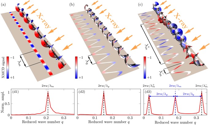
XMCD-PEEM-like numerical experiments with magnetic wires, where the x-ray beam hits the samples under the angle of 25° with respect to the surface plane. (a) The helicoidal state in a straight wire with \({{\mathcal{D}}}_{{\rm{T}}}^{{\rm{I}}}=2.7\). (b) The quasitangential state in a helical wire with \(\varkappa =0.8\), σ = 0.5, \({{\mathcal{D}}}_{{\rm{T}}}^{{\rm{I}}}=0\), \({\mathcal{C}}=+1\). (c) The periodical state with \(\varkappa =0.8\), σ = 0.5, \({{\mathcal{D}}}_{{\rm{T}}}^{{\rm{I}}}=2.7\), \({\mathcal{C}}=+1\). Colors of the surface of the magnetization rotation and the XMCD-PEEM-like contrast are equal and reveal the magnetization parallel (red) and antiparallel (blue) to the x-ray beam. (d1–d3) Fourier spectra of the XMCD-PEEM-like signal along the wires for the helicoidal, quasitangential and periodical states, respectively.

Accessing spin textures of geometrically curved magnetic thin films39,41,42,43,44, hollow cylinders37,40,45,46,47,48,49,50 and wires35,51,52,53,54 has become now a dynamic research field23,55. In our work, we performed a detailed study of the interplay between the intrinsic and extrinsic chiral interactions of 3D curvilinear objects within a 1D anisotropic Heisenberg magnet with intrinsic DMI. We established that the chiral properties of the magnetic system are necessarily determined by a single vector of the mesoscale DMI. The mDMI is a result of the interplay between intrinsic spin-orbit- and extrinsic curvature-driven DMI terms and depends both on the material and geometrical parameters. We illustrated our approach on the example of a helix wire. By changing material and geometrical parameters we identified and investigated two stationary states: homogeneous quasitangential and periodical elliptic helicoidal states. Similarly to the case of straight wire with biaxial anisotropy, the periodical domain wall state appears near the boundary between two phases as a metastable state. We proposed an approach how these states could be verified in experiments based on integral and microscopic observations. The appearance of each state can be determined by measuring of the average values of the magnetization components and/or by establishing space Fourier spectra of the coordinate-dependent magnetic signals from nanohelices. Thus we propose a method to create new artificial chiral nanostructures with defined properties from standard magnetic materials by using geometrical manipulations51,55,56,57,58,59,60,61,62, which can be used in the development of the novel spintronics and spin-orbitronics devices. In this respect, the great development in nanotechnology, e.g. high-quality thin films growing approach, glancing angular deposition technology58,62, self-assembling methods and strain engineering techniques56,57,59, gives promise that these effects can be explored experimentally. It should be emphasized, that our model could be generalized for arbitrary 1D geometry and material parameters of experimentally obtained samples, by using proper parametrization with taking into account possible coordinate dependence of material parameters. More specifically, as the experimentally realized sculptured 3D cobalt nanowires do not have any intrinsic DMI35, our theory could be applied with \({{\mathcal{D}}}^{{\rm{I}}}=0\) and predicts the homogeneously magnetized quasitangential state for the same geometry (in the limit of ultrathin wire). Subsequent theoretical study of 1D helimagnetic nanowires require investigation of non-local magnetostatical effects, field-driven switching between states with different magnetic symmetry.
Data availability
The datasets generated during and/or analysed during the current study are available from the corresponding author on reasonable request.
References
Dzyaloshinskii, I. E. Theory of helicoidal structures in antiferromagnets. i. nonmetals. Sov. Phys. JETP 19, 964–971, http://www.jetp.ac.ru/cgi-bin/e/index/e/19/4/p960?a=list (1964).
Dzyaloshinskii, I. E. The theory of helicoidal structures in antiferromagnets. II. metals. Sov. Phys. JETP 20, 223, http://www.jetp.ac.ru/cgi-bin/e/index/e/20/1/p223?a=list (1965).
Bogdanov, A., Rössler, U. & Pfleiderer, C. Modulated and localized structures in cubic helimagnets. Physica B: Condensed Matter 359–361, 1162–1164, https://doi.org/10.1016/j.physb.2005.01.303 (2005).
Rohart, S. & Thiaville, A. Skyrmion confinement in ultrathin film nanostructures in the presence of Dzyaloshinskii-Moriya interaction. Physical Review B 88, 184422, https://doi.org/10.1103/PhysRevB.88.184422 (2013).
Thiaville, A., Rohart, S., Jué, É., Cros, V. & Fert, A. Dynamics of Dzyaloshinskii domain walls in ultrathin magnetic films. EPL (Europhysics Letters) 100, 57002, https://doi.org/10.1209/0295-5075/100/57002 (2012).
Emori, S., Bauer, U., Ahn, S.-M., Martinez, E. & Beach, G. S. D. Current-driven dynamics of chiral ferromagnetic domain walls. Nature Materials 12, 611–616, https://doi.org/10.1038/nmat3675 (2013).
Ryu, K.-S., Thomas, L., Yang, S.-H. & Parkin, S. Chiral spin torque at magnetic domain walls. Nature Nanotechnology 8, 527–533, https://doi.org/10.1038/nnano.2013.102 (2013).
Bogdanov, A. N. & Yablonski, D. A. Thermodynamically stable “vortices” in magnetically ordered crystals. the mixed state of magnets. Zh. Eksp. Teor. Fiz 95, 178–182 (1989).
Ivanov, B. A., Stephanovich, V. A. & Zhmudskii, A. A. Magnetic vortices — The microscopic analogs of magnetic bubbles. J. Magn. Magn. Mater. 88, 116–120, http://www.sciencedirect.com/science/article/B6TJJ-4653NC4-R/2/4b042936c7f5ea4429c82a41bede1d8a (1990).
Bogdanov, A. N. & Hubert, A. Thermodynamically stable magnetic vortex states in magnetic crystals. J. Magn. Magn. Mater. 138, 255–269, https://doi.org/10.1016/0304-8853(94)90046-9 (1994).
Bogdanov, A. & Hubert, A. The stability of vortex-like structures in uniaxial ferromagnets. Journal of Magnetism and Magnetic Materials 195, 182–192, https://doi.org/10.1016/S0304-8853(98)01038-5 (1999).
Rößler, U. K., Bogdanov, A. N. & Pfleiderer, C. Spontaneous skyrmion ground states in magnetic metals. Nature 442, 797–801, https://doi.org/10.1038/nature05056 (2006).
Nagaosa, N. & Tokura, Y. Topological properties and dynamics of magnetic skyrmions. Nature Nanotechnology 8, 899–911, https://doi.org/10.1038/NNANO.2013.243 (2013).
Fert, A., Reyren, N. & Cros, V. Magnetic skyrmions: advances in physics and potential applications. Nature Reviews Materials 2, 17031, https://doi.org/10.1038/natrevmats.2017.31 (2017).
Dzyaloshinsky, I. A thermodynamic theory of “weak” ferromagnetism of antiferromagnetics. Journal of Physics and Chemistry of Solids 4, 241–255, http://www.sciencedirect.com/science/article/pii/0022369758900763 (1958).
Moriya, T. New mechanism of anisotropic superexchange interaction. Phys. Rev. Lett. 4, 228–230, https://doi.org/10.1103/PhysRevLett.4.228 (1960).
Fert, A. Magnetic and transport properties of metallic multilayers. Materials Science Forum 59–60, 439–480, https://doi.org/10.4028/www.scientific.net/MSF.59-60.439 (1990).
Crépieux, A. & Lacroix, C. Dzyaloshinsky–Moriya interactions induced by symmetry breaking at a surface. Journal of Magnetism and Magnetic Materials 182, 341–349, https://doi.org/10.1016/S0304-8853(97)01044-5 (1998).
Bode, M. et al. Chiral magnetic order at surfaces driven by inversion asymmetry. Nature 447, 190–193, https://doi.org/10.1038/nature05802 (2007).
Yang, H., Thiaville, A., Rohart, S., Fert, A. & Chshiev, M. Anatomy of Dzyaloshinskii-Moriya interaction at Co/Pt interfaces. Phys. Rev. Lett. 115, 267210, https://doi.org/10.1103/PhysRevLett.115.267210 (2015).
Gaididei, Y., Kravchuk, V. P. & Sheka, D. D. Curvature effects in thin magnetic shells. Phys. Rev. Lett. 112, 257203, https://doi.org/10.1103/PhysRevLett.112.257203 (2014).
Sheka, D. D., Kravchuk, V. P. & Gaididei, Y. Curvature effects in statics and dynamics of low dimensional magnets. Journal of Physics A: Mathematical and Theoretical 48, 125202, http://stacks.iop.org/1751-8121/48/i=12/a=125202 (2015).
Streubel, R. et al. Magnetism in curved geometries (topical review). Journal of Physics D: Applied Physics 49, 363001, http://iopscience.iop.org/article/10.1088/0022-3727/49/36/363001 (2016).
Yershov, K. V., Kravchuk, V. P., Sheka, D. D. & Gaididei, Y. Curvature-induced domain wall pinning. Phys. Rev. B 92, 104412, https://doi.org/10.1103/PhysRevB.92.104412 (2015).
Hertel, R. Curvature–induced magnetochirality. SPIN 03, 1340009, https://doi.org/10.1142/S2010324713400092 (2013).
Pylypovskyi, O. V. et al. Coupling of chiralities in spin and physical spaces: The Möbius ring as a case study. Phys. Rev. Lett. 114, 197204, https://doi.org/10.1103/PhysRevLett.114.197204 (2015).
Sheka, D. D., Kravchuk, V. P., Yershov, K. V. & Gaididei, Y. Torsion-induced effects in magnetic nanowires. Phys. Rev. B 92, 054417, https://doi.org/10.1103/PhysRevB.92.054417 (2015).
Yershov, K. V., Kravchuk, V. P., Sheka, D. D. & Gaididei, Y. Curvature and torsion effects in spin-current driven domain wall motion. Phys. Rev. B 93, 094418, https://doi.org/10.1103/PhysRevB.93.094418 (2016).
Pylypovskyi, O. V. et al. Rashba torque driven domain wall motion in magnetic helices. Scientific Reports 6, 23316, https://doi.org/10.1038/srep23316 (2016).
Ortix, C. Quantum mechanics of a spin-orbit coupled electron constrained to a space curve. Phys. Rev. B 91, 245412, https://doi.org/10.1103/PhysRevB.91.245412 (2015).
Kravchuk, V. P. et al. Topologically stable magnetization states on a spherical shell: Curvature-stabilized skyrmions. Phys. Rev. B 94, 144402, https://doi.org/10.1103/PhysRevB.94.144402 (2016).
Slastikov, V. V. & Sonnenberg, C. Reduced models for ferromagnetic nanowires. IMA Journal of Applied Mathematics 77, 220–235, https://doi.org/10.1093/imamat/hxr019 (2012).
Heide, M., Bihlmayer, G. & Blügel, S. Non-planar Dzyaloshinskii spirals and magnetic domain walls in non-centrosymmetric systems with orthorhombic anisotropy. Journal of Nanoscience and Nanotechnology 11, 3005–3015, https://doi.org/10.1166/jnn.2011.3926 (2011).
Bar’yakhtar, V. & Stefanovskii, E. Spectrum of spin waves in antiferromagnets with a spiral magnetic structure. Fizika Tverdogo Tela 11, 1946–1952 (1969).
Phatak, C. et al. Visualization of the magnetic structure of sculpted three-dimensional cobalt nanospirals. Nano Letters 14, 759–764, https://doi.org/10.1021/nl404071u (2014).
Mankos, M., Cowley, J. M. & Scheinfein, M. R. Quantitative micromagnetics at high spatial resolution using far-out-of-focus stem electron holography. Physica Status Solidi (a) 154, 469–504, https://doi.org/10.1002/pssa.2211540202 (1996).
Streubel, R. et al. Magnetic microstructure of rolled-up single-layer ferromagnetic nanomembranes. Advanced Materials 26, 316–323, https://doi.org/10.1002/adma.201303003 (2014).
Streubel, R. et al. Retrieving spin textures on curved magnetic thin films with full-field soft X-ray microscopies. Nat Comms 6, 7612, https://doi.org/10.1038/ncomms8612 (2015).
Streubel, R. et al. Equilibrium magnetic states in individual hemispherical permalloy caps. Appl. Phys. Lett. 101, 132419, http://aip.scitation.org/doi/10.1063/1.4756708 (2012).
Streubel, R. et al. Magnetically capped rolled-up nanomembranes. Nano Letters 12, 3961–3966, https://doi.org/10.1021/nl301147h (2012).
Ulbrich, T. C. et al. Magnetization reversal in a novel gradient nanomaterial. Phys. Rev. Lett. 96, 077202, https://doi.org/10.1103/PhysRevLett.96.077202 (2006).
Makarov, D. et al. Arrays of magnetic nanoindentations with perpendicular anisotropy. Appl. Phys. Lett. 90, 093117, http://aip.scitation.org/doi/10.1063/1.2709513 (2007).
Dietrich, C. et al. Influence of perpendicular magnetic fields on the domain structure of permalloy microstructures grown on thin membranes. Phys. Rev. B 77, 174427, https://doi.org/10.1103/PhysRevB.77.174427 (2008).
Tretiakov, O. A., Morini, M., Vasylkevych, S. & Slastikov, V. Engineering curvature-induced anisotropy in thin ferromagnetic films. Physical Review Letters 119, 077203, https://doi.org/10.1103/PhysRevLett.119.077203 (2017).
Yan, M., Kákay, A., Gliga, S. & Hertel, R. Beating the Walker limit with massless domain walls in cylindrical nanowires. Phys. Rev. Lett. 104, 057201, https://doi.org/10.1103/PhysRevLett.104.057201 (2010).
Landeros, P. & Núñez, A. S. Domain wall motion on magnetic nanotubes. Journal of Applied Physics 108, 033917, http://aip.scitation.org/doi/10.1063/1.3466747 (2010).
Otálora, J., López-López, J., Vargas, P. & Landeros, P. Chirality switching and propagation control of a vortex domain wall in ferromagnetic nanotubes. Applied Physics Letters 100, 072407, https://doi.org/10.1063/1.3687154 (2012).
Streubel, R. et al. Rolled-up permalloy nanomembranes with multiple windings. SPIN 03, 1340001, https://doi.org/10.1142/S2010324713400018 (2013).
Streubel, R. et al. Imaging of buried 3D magnetic rolled-up nanomembranes. Nano Lett. 14, 3981–3986, https://doi.org/10.1021/nl501333h (2014).
Otálora, J. A., Yan, M., Schultheiss, H., Hertel, R. & Kákay, A. Curvature-induced asymmetric spin-wave dispersion. Phys. Rev. Lett. 117, 227203, https://doi.org/10.1103/PhysRevLett.117.227203 (2016).
Smith, E. J., Makarov, D., Sanchez, S., Fomin, V. M. & Schmidt, O. G. Magnetic microhelix coil structures. Phys. Rev. Lett. 107, 097204, https://doi.org/10.1103/PhysRevLett.107.097204 (2011).
Gibbs, J. G. et al. Nanohelices by shadow growth. Nanoscale 6, 9457, https://doi.org/10.1039/c4nr00403e (2014).
Tomita, S., Sawada, K., Porokhnyuk, A. & Ueda, T. Direct observation of magnetochiral effects through a single metamolecule in microwave regions. Phys. Rev. Lett. 113, https://doi.org/10.1103/PhysRevLett.113.235501 (2014).
Kodama, T. et al. Ferromagnetic resonance of a single magnetochiral metamolecule of permalloy. Physical Review Applied 6, 024016, https://doi.org/10.1103/PhysRevApplied.6.024016 (2016).
Fernández-Pacheco, A. et al. Three-dimensional nanomagnetism. Nature Communications 8, 15756, https://doi.org/10.1038/ncomms15756 (2017).
Prinz, V. et al. Free-standing and overgrown InGaAs/GaAs nanotubes, nanohelices and their arrays. Physica E: Low-dimensional Systems and Nanostructures 6, 828–831, https://doi.org/10.1016/S1386-9477(99)00249-0 (2000).
Schmidt, O. G. & Eberl, K. Nanotechnology: Thin solid films roll up into nanotubes. Nature 410, 168–168, https://doi.org/10.1038/35065525 (2001).
Zhao, Y.-P., Ye, D.-X., Wang, G.-C. & Lu, T.-M. Novel nano-column and nano-flower arrays by glancing angle deposition. Nano Letters 2, 351–354, https://doi.org/10.1021/nl0157041 (2002).
Luchnikov, V., Sydorenko, O. & Stamm, M. Self-rolled polymer and composite polymer/metal micro- and nanotubes with patterned inner walls. Adv. Mater. 17, 1177–1182, https://doi.org/10.1002/adma.200401836 (2005).
Ureña, E. B. et al. Fabrication of ferromagnetic rolled-up microtubes for magnetic sensors on fluids. Journal of Physics D: Applied Physics 42, 055001, https://doi.org/10.1088/0022-3727/42/5/055001 (2009).
Smith, E. J., Makarov, D. & Schmidt, O. G. Polymer delamination: towards unique three-dimensional microstructures. Soft Matter 7, 11309, https://doi.org/10.1039/c1sm06416a (2011).
Mark, A. G., Gibbs, J. G., Lee, T.-C. & Fischer, P. Hybrid nanocolloids with programmed three-dimensional shape and material composition. Nature Materials 12, 802–807, https://doi.org/10.1038/nmat3685 (2013).
Acknowledgements
D.D.Sh. thanks the HZDR for kind hospitality and acknowledges the support from the Alexander von Humboldt Foundation (Research Group Linkage Programme). V.P.Kr. thanks IFW Dresden for kind hospitality and also acknowledge the support from the Alexander von Humboldt Foundation. This work is financed in part via the ERC within the EU Seventh Framework Programme (ERC Grant No. 306277) and the BMBF project GUC-LSE (federal research funding of Germany FKZ: 01DK17007).
Author information
Authors and Affiliations
Contributions
O.M.V., D.D.Sh., V.P.Kr. and U.K.R. formulated the theoretical problem. O.M.V. and D.D.Sh. performed the analytical calculations. O.M.V. performed spin-lattice simulations. O.M.V., D.D.Sh., V.P.Kr., Yu.G., U.K.R., D.M. and J.F. contributed to the discussion and writing of the manuscript text.
Corresponding author
Ethics declarations
Competing Interests
The authors declare that they have no competing interests.
Additional information
Publisher's note: Springer Nature remains neutral with regard to jurisdictional claims in published maps and institutional affiliations.
Electronic supplementary material
Rights and permissions
Open Access This article is licensed under a Creative Commons Attribution 4.0 International License, which permits use, sharing, adaptation, distribution and reproduction in any medium or format, as long as you give appropriate credit to the original author(s) and the source, provide a link to the Creative Commons license, and indicate if changes were made. The images or other third party material in this article are included in the article’s Creative Commons license, unless indicated otherwise in a credit line to the material. If material is not included in the article’s Creative Commons license and your intended use is not permitted by statutory regulation or exceeds the permitted use, you will need to obtain permission directly from the copyright holder. To view a copy of this license, visit http://creativecommons.org/licenses/by/4.0/.
About this article

Cite this article
Volkov, O.M., Sheka, D.D., Gaididei, Y. et al. Mesoscale Dzyaloshinskii-Moriya interaction: geometrical tailoring of the magnetochirality. Sci Rep 8, 866 (2018). https://doi.org/10.1038/s41598-017-18835-4
Received:
Accepted:
Published:
DOI: https://doi.org/10.1038/s41598-017-18835-4
This article is cited by
-
Chirality coupling in topological magnetic textures with multiple magnetochiral parameters
Nature Communications (2023)
-
Geometrically stabilized skyrmionic vortex in FeGe tetrahedral nanoparticles
Nature Materials (2022)
-
Building skyrmions through frustration
Nature Materials (2022)
-
Nonlocal chiral symmetry breaking in curvilinear magnetic shells
Communications Physics (2020)
Comments
By submitting a comment you agree to abide by our Terms and Community Guidelines. If you find something abusive or that does not comply with our terms or guidelines please flag it as inappropriate.
