Creation and validation of a chest X-ray dataset with eye-tracking and report dictation for AI development

Abstract

We developed a rich dataset of Chest X-Ray (CXR) images to assist investigators in artificial intelligence. The data were collected using an eye-tracking system while a radiologist reviewed and reported on 1,083 CXR images. The dataset contains the following aligned data: CXR image, transcribed radiology report text, radiologist’s dictation audio and eye gaze coordinates data. We hope this dataset can contribute to various areas of research particularly towards explainable and multimodal deep learning/machine learning methods. Furthermore, investigators in disease classification and localization, automated radiology report generation, and human-machine interaction can benefit from these data. We report deep learning experiments that utilize the attention maps produced by the eye gaze dataset to show the potential utility of this dataset.

Measurement(s)	chest X-ray image • radiologist’s dictation audio data • radiologist’s eye gaze coordinates data
Technology Type(s)	eye tracking device • machine learning • Radiologist • Chest Radiography
Sample Characteristic - Organism	Homo sapiens

Machine-accessible metadata file describing the reported data: https://doi.org/10.6084/m9.figshare.14035613

Background & Summary

In recent years, artificial intelligence (AI) has been extensively explored for enhancing the efficacy and efficiency of the radiology interpretation and reporting process. As the current prevalent paradigm of AI is deep learning, many of the works in AI for radiology use large data sets of labeled radiology images to train deep neural networks to classify images according to disease classes. Given the high labor cost of annotating images with the areas depicting the disease, large public training datasets often come with global labels describing the whole image^1,2 without localized annotation of the disease areas. The deep neural network model is trusted with discovering the relevant part of the image and learning the features characterizing the disease. This limits the performance of the resulting network. Furthermore, the black-box nature of deep neural networks and lack of local annotations means that the process of developing disease classifiers does not take advantage of expert’s knowledge of disease appearance and location in medical images. The result is a multi-layer and nonlinear model with serious concerns with respect to the explainability of its output. Another well-studied concern is the generalization capability (i.e., when the model is deployed to infer the class labels for images from other sources or distributions) and how deep neural networks are affected by scanner differences and/or demographic changes³.

In the past five decades eye-tracking has been extensively used in radiology for education, perception understanding, and fatigue measurement (example reviews^4,5,6,7:). More recently, efforts^8,9,10,11 have used eye-tracking data to improve segmentation and disease classification in Computed Tomography (CT) by integrating them in deep learning techniques. With such evidence and with the lack of public datasets that capture eye gaze data in the chest X-Ray (CXR) space, we present a new dataset that can help improve the way machine learning models are developed for radiology applications and we demonstrate its use in some popular deep learning architectures.

This dataset consists of eye gaze information recorded from a single radiologist interpreting frontal chest radiographs. Dictation data (audio and timestamped text) of the radiology report reading is also provided. We also generated bounding boxes containing anatomical structures on every image and share them as part of this dataset. These bounding boxes can be used in conjunction with eye gaze information to produce more meaningful analyses.

We present evidence that this dataset can help with two important tasks for AI practitioners in radiology:

• The coordinates marking the areas of the image that a radiologist looks at while reporting a finding provide an approximate region of interest/attention for that finding. Without altering a radiologist’s routine, this approach presents an inexpensive and efficient method for generating a locally annotated collection of images for training machine learning algorithms (e.g., disease classifiers). Since we also share the ground truth bounding boxes, the validity of the eye-tracking in marking the location of the finding can be further studied using this dataset. We demonstrate the utilization of eye gaze in deep neural network training and show that performance improvements can be obtained.

• Tracking of the eyes can characterize how radiologists approach the task of reading radiographs. The study of the eye gaze of radiologists while reading normal and disease radiographs, presented as attention maps, reveals a cognitive workflow pattern that AI developers can use when building their models.

We invite researchers in the radiology community who wish to contribute to the further development of the dataset to contact us.

Methods

Figure 1 provides an overview of the study and data generation process. In this work we use the publicly available MIMIC-CXR Database^2,12 in conjunction with the publicly available Emergency Department (ED) subset of the MIMIC-IV Clinical Database¹³. The MIMIC-IV-ED subset contains clinical observations/data and outcomes related to some of the CXR exams in the MIMIC-CXR database. Inclusion and exclusion criteria were applied to the patient attributes and clinical outcomes (via the discharge diagnosis, a.k.a the ICD-9 code) recorded in the MIMIC-IV Clinical Database¹³, resulting in a subset of 1,083 cases that equally cover 3 conditions: Normal, Pneumonia and Congestive Heart Failure (CHF). The corresponding CXR images of these cases were extracted from the MIMIC-CXR database². A radiologist (American Board of Radiology certified with over 5 years of experience) performed routine radiology reading of the images using the Gazepoint GP3 Eye Tracker¹⁴ (i.e., eye-tracking device), Gazepoint Analysis UX Edition software¹⁵ (i.e., software for performing eye gaze experiments), a headset microphone, a desktop computer and a monitor (Dell S2719DGF) set at 1920 × 1080 resolution. Radiology reading took place in multiple sessions (i.e., 30 cases per session) over a period of 2 months (i.e., March – May 2020). The Gazepoint Analysis UX Edition¹⁵ exported video files (.avi format) containing eye fixations and voice dictation of radiologist’s reading along with spreadsheets (.csv format) containing eye tracker’s recorded eye gaze data. The audio was extracted from the video files and saved in wav and mp3 format. Subsequently, these audio files were processed with speech-to-text software (i.e., https://cloud.google.com/speech-to-text) to extract text transcripts along with dictation word time-related information (.json format). Furthermore, these transcripts were manually corrected. The final dataset contains the raw eye gaze signal information (.csv), audio files (.wav,.mp3) and transcript files (.json).

Fig. 1

Flowchart of Study.

Ethical statement

The source data from the MIMIC-CXR and MIMIC-IV databases have been previously de-identified, and the institutional review boards of the Massachusetts Institute of Technology (No. 0403000206) and Beth Israel Deaconess Medical Center (2001-P-001699/14) both approved the use of the databases for research. We have also complied with all relevant ethical regulations regarding the use of the data for our study.

Data preparation

Inclusion and exclusion criteria

Figure 2 describes the inclusion/exclusion criteria used to generate this dataset. These criteria were applied to the MIMIC-IV Clinical Database¹³ to identify the CXR studies of interest. The studies were used to extract their corresponding CXR images from the MIMIC-CXR Database².

Fig. 2

Sampling flowchart for selecting images for this study from the MIMIC-IV (the ED subset) and the MIMIC-CXR datasets.0^2,13.

We selected two clinically prevalent and high impact diseases, pneumonia and congestive heart failure (CHF), in the Emergency Department (ED) setting. We also picked normal cases as a comparison class. Unlike related CXR labeling efforts¹, where the same labels are derived from radiology reports using natural language processing (NLP) alone, the ground truth for our pneumonia and CHF class labels were derived from unique discharge ICD-9 codes (verified by our clinicians) from the MIMIC-IV-ED tables¹³.

This ensures the ground truth is based on a formal clinical diagnosis and is likely to be more reliable, given that ICD-9 discharge diagnoses are typically derived from a multi-disciplinary team of treating providers after having considered all clinically relevant information (e.g., bedside observations, labs) in addition to the CXR images. This is particularly important since CXR observations alone may not always be specific enough to reach a pneumonia or CHF clinical diagnosis. The normal class is determined by excluding any ICD-9 codes that may result in abnormalities visible on CXRs and also having no abnormal labels extracted from the relevant CXR reports using CXR report labeler¹⁶. The code to run the inclusion and exclusion criteria is available on our Github repository https://github.com/cxr-eye-gaze/eye-gaze-dataset.

In addition, our sampling criteria prioritized the strategy for getting a good number of examples of disease features across a range of ages and sex from the source ED population. The goal is to support building and evaluation of computer vision algorithms that do not overly rely on age and sex biases, which may depict prominent visual features¹⁷, to predict disease classes.

Preparation of images

Preparation of images The 1,083 CXR images (Inclusion/Exclusion section) were converted from DICOM (Digital Imaging and Communications in Medicine) format to .png format: normalized (0–255), resized and padded to 1920 × 1080 to fit the radiologist’s computer’s monitor resolution (i.e., kept same aspect ratio) and to enable loading into Gazepoint Analysis UX Edition¹⁵.

A calibration image (i.e., resolution: 1920 × 1080 pixels) consisting of a white dot (30 pixels in radius) was generated (see Fig. 3 - left). The calibration image was presented to the radiologist randomly during data collection to measure eye gaze offset (see Fig. 3 - right).

Fig. 3

Calibration images presented during data collection with the radiologist’s fixation super-imposed. Left: Calibration image presented to radiologist during data collection, Right: Radiologist’s fixation super-imposed in red.

The 1,083 images and calibration images were split into 38 numbered folders (i.e., ’01’, ’02’, ’03’, …’38’) with no more than 30 images per folder. These folders were then uploaded to IBM’s internal BOXTM and shared with the radiologist who finally downloaded and loaded them to Gazepoint Analysis UX Edition software¹⁵ to perform the reading (i.e., data collection).

Data collection

Software and hardware setup

The Gazepoint GP3 Eye Tracker¹⁴ is an optical eye tracker that uses infrared light to detect eye fixation. The Gazepoint Analysis UX Edition software¹⁵ is a software suite that comes along with the Gazepoint GP3 Eye Tracker and allows performing eye gaze experiments on image series.

The Gazepoint GP3 Eye Tracker¹⁴ was set up in the radiologist’s routine working environment on a Windows desktop PC (connected at USB 3 port). The Gazepoint Analysis UX Edition software¹⁵ was also installed on the same computer. Each session was a standalone experiment that contained up to 30 images for reading by the radiologist. The radiologist’s eyes were 28 inches away from the monitor. The choice of this number of images was intentional to avoid fatigue and interruptions and to allow for timely offline review and quality assurance of each session recordings by the rest of the team. Gazepoint Analysis UX Edition software¹⁵ allows for 9-point calibration which occurred in the beginning of each session. In addition, Gazepoint Analysis UX Edition¹⁵ allows the user to move to the next image either by pressing the spacebar on the keyboard when done with a case or by waiting for a fixed time. In this way the radiologist was able to move to the next CXR image when he was done with a given image, making the experiment easier.

Radiology reading

The radiologist read 1,083 CXR images reporting in unstructured prose, same as what he would perform in his routine working environment. The goal was to simulate a typical radiology read with minimal disruption from the eye gaze data collection process. The order of the CXR images was randomized to allow a blinded radiology read. Furthermore, we intentionally withheld the reason for exam information from our radiologist in order to collect an objective CXR exam interpretation based only on the available imaging features.

The original source MIMIC-CXR Database² has the original de-identified free text reports for the same images, which were collected in real clinical scenarios where the reading radiologists had access to some patient clinical information outside the CXR image. The radiologists may even have had discussions about the patients with the bedside treating physician. Interpreting CXRs with additional patient clinical information (e.g., age, sex, other signs or symptoms) has the benefit of allowing radiologists to provide a narrower list of disease differential diagnosis by reasoning with their extra medical knowledge. However, it may also have the unintended effect of narrowing the radiology finding descriptions or subconsciously biasing what the radiologists look for in the image. In contrast, our radiologist only had the clinical information that all the CXRs came from an ED clinical setting.

By collecting a more objective read, we ensured that the CXR images used in this dataset have associated reports from both kinds of reading scenarios (read with and without patient clinical information). The goal is to broaden the range of possible technical and clinical research questions that future researchers working with the dataset may ask and explore.

The only clinical information that our radiologist was given when reading the CXRs in the eye gaze dataset was that the CXR exams were taken in the Emergency Department (ED) setting. The ED setting is broad and can include several common acute and chronic conditions that may be apparent on CXR images. The radiologist was blinded to the final diagnosis for the ED admission, asked to read the CXR as he would typically in an ED case, and the CXR image order was randomized to remove potential clinical patterns.

The eye gaze radiology read setting is set to contrast the routine radiology report setting under which the original MIMIC reports were collected because our intention is to add new value to the dataset. In the routine workflow, information not visible on the CXR images is often available to the radiologists. As a result, the reports are influenced by complex multimodal inference. We made our best attempt to separate the multimodal information in the eye gaze dataset. A future direction of this work is to integrate all the multimodal clinical information available in this dataset in the experiments.

We observed that pneumonia and heart failure (disease terminologies) are described much less frequently by our radiologist in his eye gaze reports, which we attribute to the effect of creating the reports with just the image information and no prior patient clinical information. In contrast, the findings such as lung opacity, which do not require additional clinical information and can be deducted based on image appearance alone, are consistent between original reports and those produced during the eye gaze experiments.

Data post-processing

At the end of each session the radiologist exported the following information from the Gazepoint Analysis UX Edition software¹⁵: (1) fixation spreadsheet (.csv) containing fixation information for each case in the session, (2) eye gaze spreadsheet (.csv) containing raw eye gaze information for each case in the session, and (3) videos files (.avi) containing audio (i.e., radiologist’s dictation) along with his eye gaze fixation heatmaps per session case (see Fig. 4). These files were uploaded and shared over IBM’s internal BOXTM subscribed service. A team member reviewed each video for any technical quality issues (e.g., corrupted file, video playback stopped abruptly, bad audio quality).

Fig. 4

Sample video exported from Gazepoint Analysis UX Edition¹⁵ showing a CXR case image with overlayed fixations.

Once data collection (i.e., 38 sessions) finished, the following post-processing tasks were performed.

Spreadsheet merging

From all sessions (i.e., folders), the fixations spreadsheets were concatenated into a single spreadsheet file: fixations.csv, and the raw eye gaze spreadsheets were concatenated into a single spreadsheet file: eye_gaze.csv. Mapping of eye gaze and fixation from the screen coordinate system to the original MIMIC image coordinate system was also performed at this stage.

Detailed descriptions of these tables are provided in the Data Records section.

Audio extraction and transcript generation

For each session video file (i.e., containing radiologist’s eye gaze fixations and dictation in .avi format, Fig. 4) the dictation audio was extracted and saved in audio.wav and audio.mp3 files. We used Google Speech-To-Text service https://cloud.google.com/speech-to-text to transcribe the audio (i.e., wav file) into text. The transcribed text was saved in transcript.json containing timestamps and corresponding words based on the API example found in https://cloud.google.com/speech-to-text/docs/async-time-offsets. Furthermore, the transcripts were corrected manually by three (3) team members (all verified by the radiologist) using the original audio. An example of a transcript json is given in the Data Records section.

Segmentation maps and bounding boxes for anatomies

Two supplemental datasets are also provided to enrich this dataset:

• Segmentation maps: Segmentation Maps Four (4) key anatomical structures per image were generated: i) left_lung.png, ii) right_lung.png, iii) mediastinum.png and iv) aortic_knob.png. These anatomical structures were automatically segmented by an internal segmentation model and then manually reviewed and corrected by the radiologist. Each image has pixel values 255 for anatomy and 0 for background. Figure 5 presents a sample case with its corresponding segmentation maps.

  Fig. 5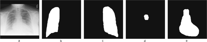

  

  Representative chest X-ray image and the corresponding segmentation maps. From Left to Right: (a) CXR image, (b) Right lung, (c) Left lung, (d) Aortic knob and (e) Mediastinum.

• Bounding boxes: An extension of a bounding box extraction pipeline¹⁸ was used to extract 17 anatomical bounding boxes for each CXR image, which include: ‘right lung’, ‘right upper lung zone’, ‘right mid lung zone’, ‘right lower lung zone’, ‘left lung’, ‘left upper lung zone’, ‘left mid lung zone’, ‘left lower lung zone’, ‘right hilar structures’, ‘left hilar structures’, ‘upper mediastinum’, ‘cardiac silhouette’, ‘trachea’, ‘right costophrenic angle’, ‘left costophrenic angle’, ‘right clavicle’, ‘left clavicle’. These zones cover the clinically most important anatomies on a Posterior Anterior (PA) CXR image. These automatically produced bounding boxes were manually corrected (when required). Each bounding box is described by the top left corner point (X_X1, Y_Y1) and bottom right corner point (X_X2, Y_Y2) on the original CXR image coordinate system. Figure 6 shows an example of anatomical bounding boxes. The information for bounding boxes of the 1,083 images are contained in bounding_boxes.csv.

  Fig. 6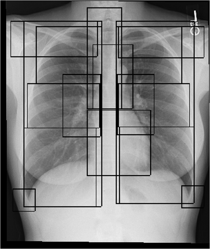

  

  Sample CXR case with 17 overlaying anatomical bounding boxes. The anatomies in the chest overlay one another on CXRs since the image is the 2D X-ray shadow capture of a 3D object.

Researchers can utilize these two (2) supplemental datasets to improve segmentation and disease localization algorithms by combining them with the eye gaze data. In the Statistical analysis on fixations subsection we utilize the bounding_boxes.csv to perform statistical analysis between fixations and condition pairs.

Data Records

An overview of the released dataset with their relationships is provided in Fig. 7. Specifically, four (4) data documents and one (1) folder are provided:

• 1. master_sheet.csv: Spreadsheet containing MIMIC DICOM ids along with study clinical indication sentence, report derived finding labels, and ICD-9 derived outcome disease labels.

• 2. eye_gaze.csv: Spreadsheet containing raw eye gaze data as exported by Gazepoint Analysis UX Edition software¹⁵.

• 3. fixations.csv: Spreadsheet containing fixation data as exported by Gazepoint Analysis UX Edition software¹⁵.

• 4. bounding_boxes.csv: Spreadsheet containing bounding box coordinates for key frontal CXR anatomical structures.

• 5. audio_segmentation_transcripts: Folder containing dictation audio files (i.e., mp3, wav), transcript file (i.e., json), anatomy segmentation mask files (i.e., png) for each dicom id.

Fig. 7

Overview of Dataset.

The dataset is hosted at https://doi.org/10.13026/qfdz-zr67¹⁹. To utilize the dataset, the only requirement for the user is to obtain Physionet access to the MIMIC-CXR Database² in order to download the original MIMIC CXR images in DICOM format. The dicom-id tag found throughout all the dataset documents maps records to the MIMIC CXR images. A detailed description of each data document is provided in the following subsections.

Master spreadsheet

The master spreadsheet (master_sheet.csv) provides the following key information:

• The dicom-id column maps each row to the original MIMIC CXR image as well as the rest of the documents in this dataset.

• The study-id column maps the CXR image/dicom to the associated CXR report, which can be found from the source MIMIC-CXR dataset².

• For each CXR study (study-id), granular radiology ‘finding’ labels have been extracted from the associated original MIMIC reports by two different NLP pipelines – first is the CheXpert NLP pipeline¹, and second is an NLP pipeline developed internally¹⁶.

• Additionally, for each CXR study (study-id), the reason for exam indication has been sectioned out from the original MIMIC CXR reports. The indication sentence(s) tend to contain patient clinical information that may not otherwise be visible from the CXR image alone.

Table 1 describes in detail each column found in the master spreadsheet.

Table 1 Master Spreadsheet.

Fixations and eye gaze spreadsheets

The eye gaze information is stored in two (2) files: a) fixations.csv, and b) eye_gaze.csv. Both files were exported by the Gazepoint Analysis UX Edition software¹⁵. Specifically, the eye_gaze.csv file contains one row for every data sample collected from the eye tracker, while fixations.csv file contains a single data entry per fixation. The Gazepoint Analysis UX Edition software¹⁵ generates the fixations.csv file from the eye_gaze.csv file by averaging all data within a fixation to estimate the point of fixation based on the eye gaze samples, stopping when a saccade is detected. Table 2 describes in detail each column found in the fixations and eye gaze spreadsheets.

Table 2 Fixations and Eye Gaze Spreadsheets.

Bounding boxes spreadsheet

The bounding boxes spreadsheet contains the following information:

• dicom_id: DICOM ID as provided in MIMIC-CXR Database² for each image.

• bbox_name: These are the names for the 17 rectangular anatomical zones that bound the key anatomical organs on a frontal CXR image. Each lung (right and left) is bounded by its own bounding box, as well as subdivided into common radiological zones (upper, mid and lower lung zones) on each side. The upper mediastinum and the cardiac silhouette (heart) bounding boxes make up the mediastinum anatomy. The trachea is a bounding box that includes the visible tracheal air column on a frontal CXR, as well as the beginnings of the right and left main stem bronchi. The left and right hilar structures contain the left or right main stem bronchus as well as the lymph nodes and blood vessels that enter and leave the lungs in the hilar region. The left and right costophrenic angles are key regions to assess for abnormalities on a frontal CXR. The left and right clavicles can have potential fractures to rule out, but are also important landmarks to assess whether the patient (hence the anatomies on the CXRs) is rotated or not (which affects the appearance of potential abnormalities). Some of the bounding boxes (e.g clavicles) could be missing for an image if the target anatomical structure is cut off from the CXR image’s field of view.

• x1: x coordinate for starting point of bounding box (upper left).

• y1: y coordinate for starting point of bounding box (upper left).

• x2: x coordinate for ending point of bounding box (lower right).

• y2: y coordinate for ending point of bounding box (lower right).

Please see Fig. 6 for an example of all the anatomical bounding boxes.

Audio, segmentation maps and transcripts

The audio_segmentation_transcripts folder contains subfolders for all the cases in the study with case dicom_id as name. Each subfolder contains: a) the dictation audio file (mp3, wav), b) the segmentation maps of anatomies (png), as described in Segmentation maps and bounding boxes for anatomies subsection above, and c) the dictation transcript (json). The dictation transcript.json contains the following tags:

• full_text: The full text for the transcript.

• time_stamped_text: The full text broken into timestamped phrases:

• phrase: Phrase text in the transcript.

• begin_time: The starting time (in seconds) of dictation for a particular phrase.

• end_time: The end time (in seconds) of dictation of a particular phrase.

Figure 8 shows the structure of the audio_segmentation_transcripts folder, while Fig. 9 shows a transcript json example.

Fig. 8

audio_segmentation_transcripts folder structure.

Fig. 9

Transcript example.

Technical Validation

We subjected two aspects of the released data to reliability and quality validation: eye gaze and transcripts.

The code for the validation tasks below can be found at https://github.com/cxr-eye-gaze/eye-gaze-dataset.

Validation of eye gaze data

As mentioned in the Preparation of images subsection, a calibration image was interjected randomly within the eye gaze sessions to measure the error of the eye gaze on the X- and Y- axis (Fig. 3). A total of 59 calibration images were presented throughout the data collection. We calculated the error by using the fixation coordinates of the last entry of each calibration image (i.e., the final resting fixation by the radiologist on the calibration mark). The overall average percentage error on X, Y axes was calculated with (error_X, error_Y) = (0.0089, 0.0504), and std: (0.0065, 0.0347) respectively. In pixels, the same error was: (error_X, error_Y) = (17.0356, 54.3943), with std: (12.5529, 37.4257) respectively.

Validation of transcripts

As mentioned in the Preparation of images subsection, transcripts were generated using Google Speech-to-Text https://cloud.google.com/speech-to-text on the dictation audio with timestamps per dictated word. The software produced two (2) types of errors:

• Type A: Incorrect identification of a word at a particular time stamp (please see example in Fig. 10).

  Fig. 10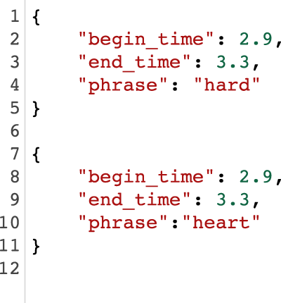

  

  Top: Example of incorrect detection. Bottom: Manual correction.

• Type B: Missed transcribed phrases of the dictation (please see example in Fig. 11).

  Fig. 11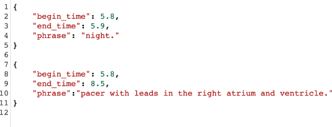

  

  Top: Missed and incorrect transcript phrase. Bottom: Manually corrected phrase.

The transcripts were manually corrected by three (3) experts and verified by the radiologist. Both types of errors were completely corrected. For Type B error, the missing text (i.e., more than one (1) word) was added with an estimation of the begin_time and end_time manually. To measure the potential error in the transcripts, the number of phrases with multiple words in a single time stamp was calculated (i.e., Type B error):

• Total number of phrases: 19,499

• Number of phrase with single words: 18,434

• Number of phrases with multiple words: 1,065

$${\rm{Type}}\,{\rm{B}}\,{\rm{error}}=1-\frac{1065}{19499}=5.46{\rm{ \% }}$$

Statistical analysis on fixations

We performed t-test analysis to measure any significant differences between fixations for each condition within anatomical structures. More specifically, we performed the following steps:

• 1. We examined the average number of fixations made in each disease condition, and found that the expert made significantly more overall fixations in the two diseased conditions than in the normal condition (p < 0.01).

• 2. For each image we calculated the number of fixations that their coordinates (i.e., X_ORIGINAL, Y_ORIGINAL in fixations.csv) fall into each anatomical zone (bounding box) found in bounding_boxes.csv.

• 3. We performed t-test for each anatomical structure between condition pairs: i) Normal vs. Pneumonia, ii) Normal vs. CHF, iii) Pneumonia vs CHF.

Figure 12 shows the duration of fixations per image for each disease condition and anatomical area, while Table 3 shows p-values from each t-test. Fixations on Normal images are significantly different from Pneumonia and CHF. More fixations are made for images associated with either the Pneumonia or CHF final diagnoses. Moreover, fixations for the abnormal cases are mainly concentrated in anatomical regions (i.e., lungs and heart) that are relevant to the diagnosis, rather than distributed at random. Overall, the fixations on Pneumonia and CHF are comparatively similar, although still statistically different (e.g., Left Hilar Structure, Left Lung, Cardiac Silhouette, Upper Mediastinum). These statistical differences demonstrate that the radiologist’s eye-tracking information provides insight into the condition of the patient, and shows how a human expert pays attention to the relevant portions of the image when interpreting a CXR exam. The code to replicate the t-test analysis can be found on our Github repository (https://github.com/cxr-eye-gaze/eye-gaze-dataset).

Fig. 12

Fixations vs. anatomical structures vs. conditions.

Table 3 p-values (at 3 decimal places) for each pair of condition and anatomy. p-values in bold demonstrate statistical significant differences.

Usage Notes

The dataset is hosted at https://doi.org/10.13026/qfdz-zr67¹⁹ The user is also required to apply for access to MIMIC-CXR Database² to download the images used in this study. Our Github repository (https://github.com/cxr-eye-gaze/eye-gaze-dataset) provides a detailed description and source code (Python scripts) on how to use this dataset and reproduce the published validation results (e.g., post-processing, machine learning experiments, etc.). The data in the MIMIC dataset has been previously de-identified, and the institutional review boards of the Massachusetts Institute of Technology (No. 0403000206) and Beth Israel Deaconess Medical Center (2001-P-001699/14) both approved the use of the database for research.

Use of the dataset in machine learning

To demonstrate the effectiveness and richness of the information provided in this dataset, we performed two sets of machine learning multi-class classification experiments, with models designed to leverage the eye gaze data. These experiments are provided as dataset applications with simple and popular network architectures and they can function as a starting point for researchers.

Both experiments used the eye gaze heatmap data to predict the multi-class classification of the aforementioned classes (i.e., Normal, CHF, Pneumonia in Table 1) and compare model performances with and without the eye gaze information. Our evaluation metric was AUC (Area Under the ROC Curve). The first experiment incorporates information from the temporal eye gaze fixation heatmaps while the second experiment utilizes static eye gaze fixation heatmaps. In contrast to temporal fixation heatmaps, static fixation heatmaps are the aggregation of all the temporal fixations into a single image.

Temporal heatmaps experiment

The first model consists of a neural architecture, where the image and the temporal fixation heatmap representations are concatenated before the final prediction layer. We denote an instance of this dataset as X⁽ⁱ⁾, which includes the image ${X}_{CRX}^{(i)}$ and the sequence of m temporal fixation heatmaps ${X}_{\mathrm{eyegaze}}^{\mathrm{(i)}}=\{{X}_{j}^{\mathrm{(i)}}{\}}_{\mathrm{k=1}}^{m}$, where k ∈ {1, …, m} is the temporal heatmap index. To acquire a fixed vector CRX representation ${{\bf{v}}}_{CRX}^{(i)}$, the image is passed through a convolutional layer with 64 filters of kernel size 7 and stride 2, followed by max-pooling, batch normalization and a dense layer of 64 units. The baseline model consists of the aforementioned image representation layer, combined with a final linear output layer that produces the classification prediction. Additionally, for the eye gaze, each heatmap is passed through a similar convolutional encoder and then the sequence of heatmaps is summarized with a 1-layer bidirectional LSTM with self-attention^20,21. We denote the heatmap representation as ${{\bf{u}}}_{eyegaze}^{(i)}$. Here, the image and heatmaps representations are concatenated before passed through the final classification layer. Figure 13 shows the full architecture. We train with Adam²², 0.001 initial learning rate and triangular schedule with fixed decay²³, 16 batch size and 0.5 dropout²⁴. The experimental results in Fig. 14 show that incorporating eye gaze temporal information, without any preprocessing, filtering or feature engineering, results in 5% AUC improvement for this prediction task when compared to the baseline model with just CXR image data as input.

Fig. 13

Model architecture for leveraging temporal eye gaze information.

Fig. 14

Experimental results with and without temporal eye gaze information, i.e., (a). Temporal model versus (b). Baseline.

Static heatmaps experiment

The previous section demonstrated performance improvements over baselines, originating from the use of temporal fixation heatmaps on a simple network architecture. In this experiment, we pose the classification problem in the U-Net architecture framework²⁵ with an additional multi-class classification block at the bottleneck layer (see Fig. 15). The encoding and bottleneck arm of the U-Net can be any standard pre-trained classifier without the fully connected layer. The two combined will act as a feature encoder for the classifier. The CNN decoder part of the network runs deconvolution layers to predict the static eye gaze fixation heatmaps. The advantage is that we can jointly train to output the eye gaze static fixation heatmap as well as predict the multi-class classification. Then, during testing on unseen CXR images, the network can predict the disease class and produce a probability heatmap of the most important locations pertaining to the condition.

Fig. 15

Block diagram of U-Net utilizing the static heatmap combined with a classification head.

We used a pre-trained EfficientNet-b0²⁶ as the encoder and bottleneck layers. The classification head was an adaptive average pooling followed by flatten, dropout²⁴ and linear output layers. The decoder CNN consisted of three convolutions followed by upsampling layers. The loss function was a weighted combination (γ) of the classification and the segmentation losses both of which used a binary cross-entropy loss function. The baseline network consisted of just the encoder and the bottleneck arm followed by the classification head.

The hyperparameter tuning for both the U-Net and the baseline classifier was performed using the Tune library²⁷ and the resulting best performing hyperparameter combination is shown in Table 4. Figure 16 shows the U-Net and baseline AUCs. Both had similar performance. However, for this experiment, we are interested in seeing how network interpretability improved with the use of static eye gaze heatmaps. Figure 17 shows a qualitative comparison of the GradCAM²⁸. The GradCAM approach is one of the common methods to visualize activation maps of convolutional networks. While the GradCAM-based heatmaps don’t clearly highlight the disease locations, we see clearly that the heatmap probability outputs of the U-Net highlight similar regions to what the static eye gaze heatmap shows.

Table 4 Best performing hyper-parameters used for the static heatmap experiments found using the Tune²⁷ library.

Fig. 16

AUC results with (a). U-Net and (b). Baseline classifier using static eye gaze information.

Fig. 17

Qualitative comparison of the interpretability of U-Net based probability maps in comparison with GradCAM for a few example use cases. (a) CHF. The physician’s eye gaze tends to fall on the enlarged heart and hila, as well as generally on the lungs, (b) Pneumonia. The physician’s eye gaze predictably focuses on the focal lung opacity and (c). Normal. Because the lungs are clear, the physician’s eye gaze skips around the image without focus.

With both experiments, we tried to demonstrate different use cases of the eye gaze data into machine learning. With the first experiment, we wanted to show how eye gaze data can be utilized in a human-machine setting where radiologist’s eye gaze information is fed into the algorithm. The second experiment shows how eye gaze information can be used for explainability purposes through generating verified activation maps. We intentionally did not include other modalities (audio, text) because of the complexity of such experiments and the scope of this paper (i.e., dataset description). We hope that these experiments can serve as a starting point for researchers to explore novel ways to utilize this multimodal dataset.

Limitations of Study

Although this study provides a unique large research dataset, we acknowledge the following limitations:

• 1. The study was performed with a single radiologist. This can certainly bias the dataset (lacks inter-observer variability) and we aim to expand the data collection with multiple radiologists in the future. However, given the relatively large size and richness of data from various sources, i.e., multimodal, we believe that the current dataset already holds great value to the research community. Given the availability of the images and our code, researchers (including our team) can expand the dataset with more reads per image in the future. In addition, we have shown with preliminary machine learning experiments that a model trained to optimize on a radiologist’s eye-tracking pattern has improved diagnostic performance as compared to a baseline model trained with weak image-level labels.

• 2. The images used during the radiology reading were in ‘png’ format and not in DICOM. That’s because the Gazepoint Analysis UX Edition¹⁵ doesn’t support DICOM format. This had the shortcoming that the radiologist could not utilize windowing techniques. However, the png images were prepared using the windowing information in the original DICOM images.

• 3. This dataset includes only Posterior Anterior (PA) CXR images as selected from the inclusion/exclusion criteria (Fig. 2). This view position criterion was clinically chosen because of its higher quality images compared to Anterior Posterior (AP) CXR images. Therefore, any analysis (e.g., machine learning models trained on only this dataset) may suffer from generalizability to AP CXR images.

References

Irvin, J. et al. Chexpert: A large chest radiograph dataset with uncertainty labels and expert comparison. Proceedings of the AAAI Conference on Artificial Intelligence 33, 590–597 (2019).
Johnson, A. E. et al. MIMIC-CXR, a de-identified publicly available database of chest radiographs with free-text reports. Scientific Data 6 (2019).
Bluemke, D. A. et al. Assessing Radiology Research on Artificial Intelligence: A Brief Guide for Authors, Reviewers, and Readers-From the Radiology Editorial Board. Radiology 294, 487–489 (2020).
Waite, S. A. et al. Analysis of perceptual expertise in radiology–Current knowledge and a new perspective. Frontiers in human neuroscience 13, 213 (2019).
Van der Gijp, A. et al. How visual search relates to visual diagnostic performance: a narrative systematic review of eye-tracking research in radiology. Advances in Health Sciences Education 22, 765–787 (2017).
Krupinski, E. A. Current perspectives in medical image perception. Attention, Perception, & Psychophysics 72, 1205–1217 (2010).
Tourassi, G., Voisin, S., Paquit, V. & Krupinski, E. Investigating the link between radiologists’ gaze, diagnostic decision, and image content. Journal of the American Medical Informatics Association 20, 1067–1075 (2013).
Khosravan, N. et al. A collaborative computer aided diagnosis (C-CAD) system with eye-tracking, sparse attentional model, and deep learning. Medical image analysis 51, 101–115 (2019).
Stember, J. N. et al. Eye Tracking for Deep Learning Segmentation Using Convolutional Neural Networks. Journal of digital imaging 32, 597–604 (2019).
Aresta, G. et al. Automatic lung nodule detection combined with gaze information improves radiologists’ screening performance. IEEE Journal of Biomedical and Health Informatics (2020).
Mall, S., Brennan, P. C. & Mello-Thoms, C. Modeling visual search behavior of breast radiologists using a deep convolution neural network. Journal of Medical Imaging 5, 035502 (2018).
Goldberger, A. L. et al. PhysioBank, PhysioToolkit, and PhysioNet: components of a new research resource for complex physiologic signals. circulation 101, e215–e220 (2000).
Johnson, A. et al. MIMIC-IV. PhysioNet https://doi.org/10.13026/A3WN-HQ05 (2020).
Gazepoint. GP3 Eye Tracker.
Gazepoint. Gazepoint Analysis UX Edition.
Wu, J. T. et al. AI Accelerated Human-in-the-loop Structuring of Radiology Reports. In AMIA (2020).
Karargyris, A. et al. Age prediction using a large chest x-ray dataset. In Mori, K. & Hahn, H. K. (eds.) Medical Imaging 2019: Computer-Aided Diagnosis, vol. 10950, 468–476, https://doi.org/10.1117/12.2512922. International Society for Optics and Photonics (SPIE, 2019).
Wu, J. et al. Automatic bounding box annotation of chest x-ray data for localization of abnormalities. In 2020 IEEE 17th International Symposium on Biomedical Imaging (ISBI), 799–803 (2020).
Karargyris, A. et al. Eye gaze data for chest x-rays. PhysioNet https://doi.org/10.13026/QFDZ-ZR67 (2020).
Cheng, J., Dong, L. & Lapata, M. Long Short-Term Memory-Networks for Machine Reading. In Proceedings of the 2016 Conference on Empirical Methods in Natural Language Processing, 551–561 (2016).
Vaswani, A. et al. Attention is all you need. In Advances in neural information processing systems, 5998–6008 (2017).
Kingma, D. P. & Ba, J. Adam: A method for stochastic optimization.
Smith, L. N. Cyclical learning rates for training neural networks. In 2017 IEEE Winter Conference on Applications of Computer Vision (WACV), 464–472 (IEEE, 2017).
Srivastava, N., Hinton, G., Krizhevsky, A., Sutskever, I. & Salakhutdinov, R. Dropout: a simple way to prevent neural networks from overfitting. The journal of machine learning research 15, 1929–1958 (2014).
Ronneberger, O., Fischer, P. & Brox, T. U-net: Convolutional networks for biomedical image segmentation. In International Conference on Medical image computing and computer-assisted intervention, 234–241 (Springer, 2015).
Tan, M. & Le, Q. V. Efficientnet: Rethinking model scaling for convolutional neural networks. arXiv preprint arXiv:1905.11946 (2019).
Liaw, R. et al. Tune: A research platform for distributed model selection and training. arXiv preprint arXiv:1807.05118 (2018).
Selvaraju, R. R. et al. Grad-cam: Visual explanations from deep networks via gradient-based localization. In Proceedings of the IEEE international conference on computer vision, 618–626 (2017).
Author information
Authors and Affiliations
Contributions
A.K. was responsible for the conceptualization, execution and management of this project. S.K. contributed to the conceptualization and was responsible for the design and execution of the use case experiments, the data and code open sourcing and preparation of the manuscript. I.L. designed the neural architecture that utilizes the temporal fixation heat maps, conducted the respective machine learning experiments, created the hyper-parameter tuning pipeline and edited the manuscript. J.W. was responsible for the clinical design of the dataset, data sampling and documentation for the project, development of the bounding box pipeline and organizing the validation of results, as well as writing and editing the manuscript.A.S. was responsible for the interpretation of images with eye-tracking, experimental design, and editing of the manuscript. M.T. contributed prior experience with eye-tracking studies, equipment, and methodologies, and assisted with the analysis. S.A. contributed to the conceptualization and was responsible for data collection and processing. D.B. contributed to the original team formation and consulted on eye gaze tracking technology and data collection. V.M. contributed to the initial concept review and securing funding for equipment/capital and execution of the project. E.K. contributed to the clinical design of the study. M.M. contributed to the design of experiments, supervision of the work and writing of the manuscript. All authors reviewed the manuscript.
Corresponding authors
Ethics declarations
Competing interests
The authors declare no competing interests.
Additional information
Publisher’s note Springer Nature remains neutral with regard to jurisdictional claims in published maps and institutional affiliations.
Rights and permissions
Open Access This article is licensed under a Creative Commons Attribution 4.0 International License, which permits use, sharing, adaptation, distribution and reproduction in any medium or format, as long as you give appropriate credit to the original author(s) and the source, provide a link to the Creative Commons license, and indicate if changes were made. The images or other third party material in this article are included in the article’s Creative Commons license, unless indicated otherwise in a credit line to the material. If material is not included in the article’s Creative Commons license and your intended use is not permitted by statutory regulation or exceeds the permitted use, you will need to obtain permission directly from the copyright holder. To view a copy of this license, visit http://creativecommons.org/licenses/by/4.0/.
The Creative Commons Public Domain Dedication waiver http://creativecommons.org/publicdomain/zero/1.0/ applies to the metadata files associated with this article.
About this article
Cite this article
Karargyris, A., Kashyap, S., Lourentzou, I. et al. Creation and validation of a chest X-ray dataset with eye-tracking and report dictation for AI development. Sci Data 8, 92 (2021). https://doi.org/10.1038/s41597-021-00863-5
Received:
Accepted:
Published:
DOI: https://doi.org/10.1038/s41597-021-00863-5
This article is cited by
-
Effective processing pipeline PACE 2.0 for enhancing chest x-ray contrast and diagnostic interpretability
Scientific Reports (2023)
Visual Image Annotation for Bowel Obstruction: Repeatability and Agreement with Manual Annotation and Neural Networks
Journal of Digital Imaging (2023)
REFLACX, a dataset of reports and eye-tracking data for localization of abnormalities in chest x-rays
Scientific Data (2022)