
Abstract
With the recent explosion of chemical libraries beyond a billion molecules, more efficient virtual screening approaches are needed. The Deep Docking (DD) platform enables up to 100-fold acceleration of structure-based virtual screening by docking only a subset of a chemical library, iteratively synchronized with a ligand-based prediction of the remaining docking scores. This method results in hundreds- to thousands-fold virtual hit enrichment (without significant loss of potential drug candidates) and hence enables the screening of billion molecule–sized chemical libraries without using extraordinary computational resources. Herein, we present and discuss the generalized DD protocol that has been proven successful in various computer-aided drug discovery (CADD) campaigns and can be applied in conjunction with any conventional docking program. The protocol encompasses eight consecutive stages: molecular library preparation, receptor preparation, random sampling of a library, ligand preparation, molecular docking, model training, model inference and the residual docking. The standard DD workflow enables iterative application of stages 3–7 with continuous augmentation of the training set, and the number of such iterations can be adjusted by the user. A predefined recall value allows for control of the percentage of top-scoring molecules that are retained by DD and can be adjusted to control the library size reduction. The procedure takes 1–2 weeks (depending on the available resources) and can be completely automated on computing clusters managed by job schedulers. This open-source protocol, at https://github.com/jamesgleave/DD_protocol, can be readily deployed by CADD researchers and can significantly accelerate the effective exploration of ultra-large portions of a chemical space.
Introduction
The recent expansion of make-on-demand libraries to billions of synthesizable molecules has attracted significant attention from the drug-discovery community, because such ultra-large databases provide access to novel, unchartered areas of the chemical universe1,2,3. On the other hand, the emergence of ultra-large libraries has highlighted significant limitations of conventional docking approaches that typically operate on the scale of millions of molecules. With chemical libraries comprising 100 billion molecules on the horizon4, it will soon become impossible to deploy conventional docking at its full potential, and so far, only a handful of billion-sized docking campaigns have been conducted on elite supercomputing facilities2,5.
It should also be noted, that docking is not just computationally demanding, but also a remarkably wasteful process in which a very small subset of top-scoring compounds is considered for experimental evaluation. Thus, most docked molecules are simply discarded6. To approach this challenge in the context of the global shortage of computational docking power, we have recently developed Deep Docking (DD), an artificial intelligence (AI)–driven approach that provides very economical yet highly reliable access to ultra-large docking. After the preparation of chemical library and receptor stages, DD relies on the iterative execution of five sequential stages (DD phases 1–5) that comprise ligand sampling, ligand preparation, docking, model training and inference. A final stage of docking is then performed to process the compounds that are retained by DD as prospective top-scoring molecules.
Development of DD to accelerate structure-based virtual screening
In 2006, we proposed Progressive Docking, a hybrid approach that uses information on already-docked molecules to predict the scores of yet unprocessed entries of a database with quantitative structure activity relationship models based on partial least squares regression, thus reducing the docking workload7. However, the acceleration offered by this and similar shallow-learning methods that followed8,9 was not yet sufficient to screen more than a few million compounds. To enable structure-based screening of billion-sized molecular libraries, we recently developed DD, a technique that iteratively trains deep neural networks (DNNs) with small batches of explicitly docked compounds to infer the ranking of the yet-unprocessed remainder of the library10. In this way, DD can discard unfavorable (undockable) molecular structures without wasting valuable computational resources (Fig. 1).

In the DD workflow, DNN models are trained to predict docking scores from 2D molecular fingerprints using only a very small portion (1%) of the database that needs to be docked. The score classes (top or low scoring) of the remaining molecules are then inferred rather than explicitly calculated with actual docking. In the end, only predicted best-scoring molecules remain to be conventionally docked, whereas unfavorable molecules are filtered out.
We have used the DD protocol to virtually screen the zinc is not commercial (ZINC)15 library (1.36 billion molecules)11 against 12 proteins representing four major families of drug targets10. We demonstrated that DD needs to dock only 1% of the molecules to significantly reduce (100-fold) the size of a chemical library while retrieving 90% of the best-scoring structures (virtual hits defined by the FRED scores12), and that even larger reductions can be achieved by lowering the user-defined percentage of retrieved virtual hits.
In a consecutive study, we also applied DD to screen ZINC15 against the severe acute respiratory syndrome coronavirus 2 (SARS-CoV-2) main protease (Mpro), a prominent drug target for coronavirus disease of 2019, using the Glide Single Precision (SP) approach13. The identified ‘make-on-demand’ compounds were structurally different from known protease inhibitors14. Our own experimental validation of DD-proposed hits showed that 15% were active against the target, with the established IC50 values ranging from 8 to 251 μM15,16. Specifically, this screen led to the discovery of a novel series of compounds based on a dihydro-quinolinone core that were confirmed experimentally as low micromolar Mpro inhibitors by us15,16 as well as by an independent study17. After our initial results, similar machine learning approaches have rapidly emerged that emulate (rather than explicitly compute) docking scores18,19,20,21,22, highlighting a global demand for AI-accelerated virtual screening23,24.
The current version of the DD protocol can be seamlessly integrated into existing drug-discovery pipelines that rely on popular docking programs. An automated workflow has also been developed to facilitate the adoption of DD by drug-discovery scientists with minimal or no experience in machine learning and programming.
Experimental design
Preparation of chemical libraries
The most commonly used ultra-large chemical libraries are ZINC and the ‘make-on-demand’ collections from Enamine. The ZINC15 database11 contains 1.5 billion molecules that can be readily downloaded as a whole in simplified molecular-input line-entry system (SMILES) format; it also provides access to several smaller subsets such as drug- and lead-like molecules. The library offers up to four precalculated stereoisomers per molecule and allows protomer and tautomer states to be computed at different pH ranges11. The newest version, ZINC20, has also been recently released, comprising ~1 billion molecules25. Furthermore, the Enamine REAL database26 includes 1.95 billion make-on-demand molecules that can be synthesized with an 85% average success rate. On the other hand, Enamine REAL Space27 is the largest database of commercially available compounds, accounting for 19 billion not-enumerated molecules.
Just like in the case of conventional docking, a chemical library has to be preprocessed for DD. Explicit isomeric configurations and correct ionization states need to be enumerated for each molecule. OpenEye flipper (license required)28 or rdkit’s EnumerateStereoisomers (freely available)29 are examples of programs that can be used to enumerate isomers, while tautomers and protonation states can be calculated by various licensed (e.g., QUACPAC30 and ChemAxon (http://www.chemaxon.com)) or open-source (e.g., openbabel31 and Ambit32) software. Circular binary Morgan fingerprints33,34 with radius 2 and size of 1,024 bits, to be used as descriptors, can then be computed from the SMILES of the prepared molecules. These extended-connectivity fingerprints represent a machine-readable description of molecules based on a fixed-length binary bit vector encoding the presence or absence of specific substructures (circular atom neighborhoods at specified radius; Supplementary Fig. 1)35. The fingerprint bits are used as features for the DNN models, which aim to learn which substructures are responsible for high predicted binding affinities (in terms of docking scores). In DD, Morgan fingerprints are stored as the indexes of bits set to 1 rather than the entire fixed-length vector (Box 1), and they are decompressed to the regular 1,024-bit representation on the fly.
Receptor preparation
Target structures need to be prepared before the docking grids can be generated. Non-structural water, lipids and solvent molecules are usually removed; the target protein may require structural optimization to repair any missing parts, add hydrogens, compute correct protonation states of residues and energetically relax the structure. This optimization process can be performed with various licensed (e.g., Schrödinger36 and Molecular Operating Environment37) and free (e.g., UCSF Chimera’s Dock Prep38) program suites. The Protein Preparation Wizard tool from Maestro36 provides a straightforward and automated way to perform such preparation. Any other protein preparation tool can be used for this purpose. The generation of docking grids, on the other hand, strictly depends on the docking program that the user intends to use. In the Procedure, we outline the steps to prepare grids for docking with Glide or FRED.
Molecular sample size
Validation, test and initial training sets are randomly sampled from the entire docking library at the first DD pass. From the second iteration on, the training set is iteratively augmented with random batches of molecules classified as virtual hits in the inference stage of the previous iteration. The chosen sample size should be large enough to properly represent the chemical diversity of the investigated library. At the same time, the maximum sample size inevitably depends on the total amount of docking (number of docked compounds) that is feasible on the user’s system.
Validation and test sets are generated only in the first iteration. Because the score threshold used to define virtual hits is decreased at each DD iteration, using small-sized sets can cause generalization issues, especially in the last iteration, in which the number of positive samples in the two sets is very limited (e.g., 0.01%). This problem might be difficult to diagnose, because the phenomenon may not be detectable in earlier iterations when positive samples are sufficiently well represented. We recommend choosing the size of validation and test sets in the first iteration as large as possible, ideally comprising 1 million molecules each, and absolutely avoiding using less than 250,000 molecules (corresponding to 25 positive samples in the last iteration), because we have observed that those values are sufficient to obtain robust and generalizable docking models for libraries that contain on the order of 1 billion compounds10. If at any iteration the number of virtual hits in the validation or test set is ≤10, model training is automatically canceled by the program.
The size of the training set, on the other hand, influences mainly model precision, and performances improve with larger training sets (700,000–1,000,000 molecules) and more iterations (8–11). If deep learning–dedicated resources available to the user (such as graphics processing units (GPUs)) are limited, we recommend using larger training sets for a smaller number of iterations (for at least four iterations) rather than the alternative, because the resulting models, although usually showing slightly worse performances, require fewer iterations of training and inference to achieve an acceptable result. An example is reported in Fig. 2, illustrating the effect of different training set size and number of iterations on a DD run against the dimerization site of the androgen receptor (Protein Data Bank (PDB) ID: 1R4I39). Performing the same total amount of docking (~4,200,000 molecules including validation and test set), the four-iteration (depicted in light green) strategy using a training size of 700,000 returned a final number of qualified molecules slightly higher than the eight-iteration (depicted in violet) strategy (~58 million versus ~49 million); however, it required half the training and inference computations. Thus, it may be a better choice for systems with a limited number of GPUs. On the other hand, the use of a larger training set (700,000 molecules) for the same number of DD iterations (four) substantially improved the DD reduction performances (~58 million versus ~108 million qualified molecules obtained by using a training size of 350,000, depicted in dark pink). If the resources for docking are limited, we recommend choosing an initial training sample size equal to the maximum number of molecules that can be docked with the user’s system (ideally 1,000,000) and dock it, and then use the procedure outlined at Step 23B of Procedure 1 or 10B of Procedure 2 to identify a value that provides an optimal balance between amount of docking and model performance for the user’s specific system and that can be used in successive iterations.

Initial validation and test sets were of 700,000 molecules in all three cases. The final number of qualified molecules was ~58 million for the four-iteration/700,000-molecule training size run (light green), ~108 million for the four-iteration/350,000-molecule training size run (dark pink) and ~49 million for the eight-iteration/350,000-molecule training size run (violet). K, thousand; M, million.
Model training and inference
Each iteration step in the DD protocol encompasses model training and inference. To identify virtual hits, the protocol uses binary classifiers in the form of feedforward DNN models (multilayer perceptrons) trained on 1,024-bit circular Morgan fingerprints. Binary ‘positive samples’ in training, validation and test sets are virtual hits with scores above a threshold, corresponding to a predefined top percentage of the docking-ranked molecules in the validation set. The rest of the molecules are labeled as ‘negative samples’. These top-percentage values can be specified by the user for the first and the last iterations, whereas for the intermediate ones, the value will be linearly changing between those two.
After the binary labels are generated, a user-specified number of models with different combinations of hyperparameters (number of hidden layers and neurons, dropout frequencies, oversampling of minority class and class weights) are trained to optimize model test set accuracy by using a grid search strategy.
After the training phase is finished for the initial iteration, the optimal binary classifier is used for inference of virtual hit-likeness of the remainder of the molecular library. For the next iterations, training, validation and test sets are augmented with new compounds randomly selected from molecules with predicted virtual hit-likenesses higher than a classification threshold corresponding to a user-defined recall value for validation predictions. This recall value is a critical parameter, which, if set too high, may significantly increase the number of remaining molecules. On the other hand, if the recall is set too low, large portions of virtual hits may be discarded. Thus, we recommend setting the recall between 0.75 and 0.90 (corresponding to 75% and 90% retrieved virtual hits, respectively).
It is important to note that virtual hit calling becomes more stringent as the top-percentage threshold value is decreased linearly with the number of iterations; thus, the definition of ‘positive’ and ‘negative’ labels also changes at each iteration for all molecules in the training, validation and test sets. The inference is always performed over the whole library, usually setting the initial percentage value for virtual hit selection to 1% and the final value to 0.01%. The total number of iterations typically ranges from 4 to 11, and we normally train 24 models at each iteration in the optimization step. For most docking campaigns, these parameters are sufficient to shrink a database of 1–1.5 billion molecules to a few million compounds that could be conventionally docked with regular computational resources. Alternatively, as we mentioned before, the preset recall value could be adjusted for more ‘aggressive’ DD-selection of top-scored compounds.
Applications
The DD protocol can be used in conjunction with any popular docking program. In our DD campaigns, we were able to dock billion-size (1B+) chemical libraries against various targets using FRED12, Glide13, Autodock-GPU40, QuickVina241 and ICM42,43 docking suites. The presented protocol explains how to set up and run DD against a generic protein target. Although the steps required for protein, ligand and docking grid preparation are explained using specific tools that we use in house, all of those can be readily adapted to similar programs and computer-aided drug discovery (CADD) packages.
Comparison with alternative methods
One of the major challenges of modern CADD is a constantly growing need for computational resources required to screen chemical libraries that are exploding in size because of recent advances in automated synthesis and robotics. Few docking packages have been proven successful for screening of 1B+ libraries by relying on their code scalability across supercomputing clusters. For example, OpenEye GigaDocking44 was used to dock the Enamine REAL database into the purine nucleoside phosphorylase and heat shock protein 90 targets in <1 d using 27,000 and 45,000 Amazon Web Services (AWS) cloud CPUs, respectively. The popular Autodock program has been parallelized for Compute Unified Device Architecture (CUDA)45 and deployed on the Summit supercomputer (comprising >27,000 GPUs) to dock the same library into the SARS-CoV-2 Mpro active site in ~1 d5. VirtualFlow2 is another automated platform for docking large libraries using supercomputing systems that has been used to screen 1.4 billion molecules in 2 weeks (using 8,000 CPUs). Very recently, Bender et al. developed a guide for ultra-large docking campaigns, highlighting that computing clusters of 500–1,000 CPU cores are required to perform billion-scale virtual screening in a timely manner46. These docking platforms achieved great high-throughput but are extremely resource demanding in comparison to DD.
Consequently, because of the computational cost, conventional docking of ultra-large libraries remains unaffordable for most of the research community. Hence, various machine learning emulation techniques of docking have been proposed to perform such tasks without large computing resources. In Supplementary Table 1, we have listed several of such methods that have been developed as a proof of concept to approximate docking scores from molecular structural features (descriptors)9,18,19,20,21,22. Although these methodologies cannot be easily compared (owing to the use of different benchmark sets and docking libraries), it is possible to stipulate that DD is one of the fastest AI-enabled docking platforms and the only method that has been extensively tested on 1B+ libraries. In addition, the DD protocol does not rely on a particular docking program, and thus it is compatible with the emerging large-scale docking methods to improve their high-throughput capabilities.
Limitations
Some technical limitations of DD that are worth mentioning are related to the extensive use of GPU acceleration. The protocol requires access to GPU resources for optimal performance, in contrast to most of the docking platforms that rely on CPUs. In addition, DD is implemented for fast and economical virtual screening and thus provides docking details exclusively for the top-scoring molecules and disregards large fractions of chemical libraries. Therefore, docking campaigns assessing hit rate variability with docking scores1 or rescoring low-ranked molecules47 should consider a brute-force approach instead. In addition, the quality of DD results entirely depends on the suitability of the docking program to prioritize active molecules from an ultra-large library. Hence, we anticipated that it would be challenging to discover active molecules from DD of a library of a billion molecules if docking performs poorly on the specific target, just like in the case of conventional docking1. In this context, recent work by Bender et al. provides useful guidelines for establishing benchmarking calculations before performing large-scale docking46.
Overview of the protocol
The present protocol provides guidance on how to set up and run a DD campaign with Glide SP and FRED docking packages. Minor modifications can be applied to adapt the same workflow to other docking programs.
We outline two alternative procedures to set up and run a DD campaign. The first relies on manually running each individual script (Procedure 1). This option is well suited for users who do not have access to large computational facilities or for those who want to use only specific DD steps in their drug-discovery campaigns.
The second option relies on a series of scripts that automatically run each stage on a cluster managed by a Simple Linux Utility for Resource Management (Slurm) job scheduler (Procedure 2). This option is particularly suitable for automation purposes and for performing virtual screening campaigns on large computational systems. Procedures 1 and 2 share a number of common steps (Supplementary Table 2). Both procedures have been extensively tested by users with no prior knowledge of the DD protocol.
Materials
Equipment
Molecular data
-
A chemical library with molecules in the SMILES format. A ready-to-screen version of ZINC20 (downloaded in early March 2021) with SMILES and already calculated fingerprints has been deposited at https://files.docking.org/zinc20-ML/
-
3D structure of the receptor in PDB format
-
An example iteration to test that the protocol can be downloaded from the Federated Research Data Repository at https://doi.org/10.20383/102.0489
Software
-
Python3.0+
-
Receptor preparation: Schrödinger Maestro suite36 or alternative program for initial protein optimization, Maestro for Glide docking grid generation, Make Receptor48 from OpenEye for FRED docking grid generation or alternative protein-preparation tools for other docking software
-
Ligand preparation: QUACPAC30 and OMEGA28 OpenEye modules or other similar programs for tautomer and protomer enumeration, stereoisomer enumeration and 3D conformer generation
-
Docking: Glide SP13 or FRED12 program; the protocol can be easily adapted to any other conventional docking program
-
Descriptor calculation and machine learning: Python3.0+ conda environment (https://docs.conda.io/en/latest) with rdkit29, tensorflow-gpu (version 1.14.0 or higher)49, pandas, numpy, keras, matplotlib and scikit-learn50 (called dd-env in the protocol). A yml file, called environment.yml, is available in the utilities folder of the repository (https://github.com/jamesgleave/DD_protocol) for setting up the environment (see https://conda.io/projects/conda/en/latest/user-guide/tasks/manage-environments.html#creating-an-environment-from-an-environment-yml-file for details)
-
DD program: all the scripts required to prepare a library and to run DD are freely available from https://github.com/jamesgleave/DD_protocol
-
Text editor
Hardware
-
Windows, Macintosh or Linux computer
-
Linux system or cluster (preferably with Slurm workload manager, https://slurm.schedmd.com/documentation.html) with CPU nodes and preferably also GPU nodes for machine learning. Our in-house setup consists of 50 GPUs (Nvidia Tesla V100 GPUs with 32 GB of memory) and 640 CPU cores (Intel Xeon Silver 4116 CPU @ 2.10 GHz)
Procedure 1: manual DD
-
1
Access the Linux system, create a DeepDocking folder and clone or copy the DD_protocol repository there. No installation is required to run the scripts.
Stage I: chemical library processing
Timing ~13 h
-
2
Download the library of SMILES in the DeepDocking folder. If the library is provided as separate files, concatenate them into a single file from the command line:
cat *smi > library.smi
-
3
Create a smiles folder and divide the library into evenly populated files of 10,000,000 molecules each, all placed inside the folder:
split -d -l 10000000 library.smi smiles/smiles_all_ --additional-suffix=.smi
This reorganization step enables one to efficiently run the random sampling and inference stages on a larger number of smaller files rather than a massive, memory-consuming library file. Because these processes are run on each file independently, any other value can be used instead of 10,000,000 to better fit specific computational setups (e.g., to have a number of files equal to the number of cores available on a node to optimize the sampling). The number of resulting files will depend on the size of the original database and the number of molecules specified for each file.
Enumerate stereoisomers, tautomers and protomers
Critical
Stereoisomers, tautomers and protomers must be enumerated using, for instance, OpenEye tools, and Morgan fingerprints must be calculated (Fig. 3). Other similar database preparation tools can be used for the same purpose. The procedure described here calculates all the possible stereoisomers of a given molecule and the dominant tautomer form (protonated at pH 7.4) for each isomer. These commands can be changed, for example, to enumerate multiple tautomers and protomers (see https://www.eyesopen.com/quacpac for guidance); each of these must be assigned a unique name, however, resulting in a substantial increase in the number of unique library entries. For some chemical libraries, the tautomers and protomers are partially or completely enumerated, and therefore these steps may not be required.
-
4
For each file generated in Step 3, enumerate stereocenters with unspecified stereochemistry using the flipper tool from the OpenEye OMEGA module, assigning a unique name to each isomer:
Fig. 3: Chemical library preparation for DD. 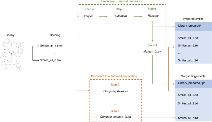
Initially, the library is obtained in SMILES format and split into evenly populated files to facilitate sampling and inference. Depending on the available resources, the user can then follow two preparation procedures. Procedure 1 (manual preparation) requires each preparation action to be executed manually (enumeration of stereoisomers, tautomers and protomers; renaming the files; and calculation of Morgan fingerprints). Procedure 2 (automated) allows running all the preparation automatically; however, it requires access to a computing cluster running with a job scheduler (Slurm). Both processes will generate a folder with the prepared SMILES and another one with the corresponding Morgan fingerprints in DD format.
flipper -in smiles/smiles_all_1.smi -out smiles/smiles_all_1_isom.smi -warts
-
5
Calculate the dominant tautomeric and protonation form of each isomer at pH 7.4 using the tautomers tool from the OpenEye QUACPAC module:
tautomers -in smiles/smiles_all_1_isom.smi -out smiles/smiles_all_1_states.smi -maxtoreturn 1 -warts false
-
6
Create a folder for the prepared files (library_prepared) and move the files generated in the previous step inside it, renaming them and changing their extension from .smi to .txt:
mv smiles/smiles_all_1_states.smi library_prepared/smile_all_1.txt

Morgan fingerprints
-
7
Activate the conda environment and use the morgan_fp.py script (provided in the utilities folder of the repository) to calculate the Morgan fingerprints of the prepared structures from their SMILES:
python morgan_fp.py --smile_folder_path ~/DeepDocking/library_prepared --folder_name ~/DeepDocking/library_prepared_fp --tot_process 60
This will create a library_prepared_fp folder with the resulting fingerprints. The tot_process argument controls how many files from library_prepared will be processed in parallel using multiprocessing.
Critical step
DD works exclusively with Morgan fingerprints of radius 2 and 1,024 bits in the format generated by the morgan_fp.py script, which is the name of the molecule followed by the indexes of fingerprint bits that are set to 1, comma separated (Box 1).
Stage II: receptor preparation
Timing ~30 min
-
8
Obtain the PDB structure of the target molecule from a public repository (e.g., the PDB51). Where possible, selecting target structures with bound ligands is recommended.
-
9
Use the Protein Preparation Wizard tool from Maestro suite36 to prepare and optimize the target structure by following the procedure illustrated at https://www.schrodinger.com/training/videos/protein-preparation. Any other protein preparation tool can be used for the same purpose.
-
10
Save the resulting optimized structure in PDB format.
-
11
Depending on the choice of docking software, the grid can be generated in different ways. Each process has been described extensively elsewhere; therefore, in the present protocol, we describe only the default workflows for Glide (A) and FRED (B). Detailed instructions on how to customize the grid generation process can be found in the training videos provided by Schrödinger for Glide (https://www.schrodinger.com/training/videos/docking-receptor-grid-generation) and in the manual of OEDocking for FRED (https://docs.eyesopen.com/applications/oedocking/make_receptor/make_receptor.html).
-
(A)
Generation of the Glide docking grid
-
(i)
Launch the Maestro graphical user interface (GUI).
-
(ii)
Load the prepared PDB in Maestro using ‘File’ → ‘Import Structures …’
-
(iii)
In the Tasks panel, search for ‘Receptor Grid Generation’ and select it.
-
(iv)
In the Receptor panel, check the ‘Pick to identify the ligand’ box and select the bound ligand in the Workspace.
-
(v)
Press ‘Run’. The docking grid will be generated in zip format.
-
(i)
-
(B)
Generation of the FRED docking grid
-
(i)
Open Make Receptor GUI.
-
(ii)
Import the prepared PDB structure using ‘File’ → ‘Open …’
-
(iii)
Check the ‘Pro’ box for the target protein and the ′Lig′ box for the ligand.
-
(iv)
Adjust the box size in the Box panel, if necessary.
-
(v)
Press ‘Create Shape’ in the Shape panel.
-
(vi)
Type the name of the protein and ligand in the respective boxes in the Finish panel and press ‘Save’ to save the grid in oeb format.
-
(i)
-
(A)
-
12
Move the grid into a docking_grid directory in the DeepDocking folder.
Stage III: random sampling of molecules in the first iteration (DD phase 1)
Timing ~15 min
-
13
In a projects directory, create a protein_test project folder. The DD process (Fig. 4) will output all the results into this folder.
Fig. 4: General DD workflow. 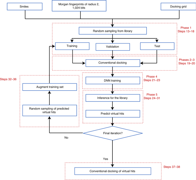
The method comprises five phases to be repeated iteratively and one final phase in which predicted virtual hits are conventionally docked to the target. Validation and test sets are generated and docked only in the first iteration. Step numbering refers to Procedure 1 (manual version).
-
14
Activate the conda environment and use the molecular_file_count_updated.py script provided in the scripts_1 folder with the following command to determine the number of molecules to sample from each library file to generate training, validation and test sets, each containing 1,000,000 molecules:
python molecular_file_count_updated.py --project_name protein_test --n_iteration 1 --data_directory ~/DeepDocking/library_prepared_fp --tot_process 60 --tot_sampling 3000000
A Mol_ct_file_updated_protein_test.csv file will be created in the ~/DeepDocking/library_prepared_fp Morgan fingerprint folder, reporting the number of molecules to sample from each file.
Critical step
The choice of molecular sample sizes in the first iteration is critical, because validation and test sets are generated only during this iteration and should be as large as possible (ideally, 1,000,000 molecules each). Refer to Experimental design for detailed information on how to properly choose the sizes of validation, test and training sets.
-
15
Use the sampling.py script to perform random sampling:
python sampling.py --project_name protein_test --file_path ~/DeepDocking/projects --n_iteration 1 --data_directory ~/DeepDocking/library_prepared_fp --tot_process 60 --train_size 1000000 --val_size 1000000
This step will create an iteration_1 folder inside the project directory and will generate three files with the names of 1,000,000 molecules each. train_size and val_size arguments control the number of molecules to sample for the training set and validation/test set files, respectively. Validation and test sets will be read always from the iteration_1 folder, regardless of the iteration.
Critical step
The sum of the train_size and 2val_size arguments must be equal to the tot_sampling value of Step 14 in the first iteration.
-
16
Remove the overlaps between sets using the sanity_check.py script:
python sanity_check.py --project_name protein_test --file_path ~/DeepDocking/projects --n_iteration 1
-
17
Extract the fingerprints of the sampled molecules:
python extracting_morgan.py --project_name protein_test --file_path ~/DeepDocking/projects --n_iteration 1 --morgan_directory ~/DeepDocking/library_prepared_fp --tot_process 60
This will create a morgan folder in the iteration directory, with three .csv files containing the fingerprints of the molecules.
-
18
Extract the corresponding SMILES:
python extracting_smiles.py --project_name protein_test --file_path ~/DeepDocking/projects --n_iteration 1 --smile_directory ~/DeepDocking/library_prepared --tot_process 60
The SMILES will be extracted into a smile folder inside the iteration directory.

Stage IV: ligand preparation (DD phase 2)
Timing ~12 h
-
19
The following procedures can be used to prepare molecules for docking with Glide SP (A) and FRED (B) using an OMEGA module (https://docs.eyesopen.com/applications/omega/). Alternative conformer generation programs can be used for the same purpose.
-
(A)
Ligand preparation for Glide docking
-
(i)
Create an sdf folder in iteration_1. Run OMEGA conformer generation in classic mode (one conformer per molecule):
oeomega classic -in smile/train_smiles_final_updated.smi -out sdf/training_sdf.sdf -maxconfs 1 -strictstereo false -mpi_np 60 -log training.log -prefix conf_training
for each smi file inside the smile folder.
-
(i)
-
(B)
Ligand preparation for FRED docking
-
(i)
Go to the iteration_1 directory and create an sdf folder. Run OMEGA 3D conformer generation in pose mode:
oeomega pose -in smile/train_smiles_final_updated.smi -out sdf/training_sdf.oeb.gz -strictstereo false -mpi_np 60 -log training.log -prefix conf_training
for each file inside the smile folder. When running in pose mode, OMEGA will output a ligand-dependent number of 3D conformations for each molecule in a oeb.gz file in the sdf folder.
-
(i)
-
(A)
Stage V: molecular docking (DD phase 3)
Timing ~20 h
-
20
Docking of the sampled molecules can be performed using Glide SP (https://www.schrodinger.com/products/glide) (A) or FRED (https://docs.eyesopen.com/applications/oedocking/fred/fred.html) (B) or any other docking program:
-
(A)
Glide SP docking
-
(i)
From scripts_1, run:
python input_glide.py --project_name protein_test --file_path ~/DeepDocking/projects --grid_file ~/DeepDocking/docking_grid/glide_grid.zip --iteration_no 1 --glide_input ~/DeepDocking/DD_protocol/scripts_1/glide_template.in
to create a docked folder in iteration_1 and generate a docking input script for each file in the sdf folder. Note that input_glide.py will modify only the GRIDFILE and LIGANDFILE line of the glide_template.in script in scripts_1, whereas all the other docking parameters will be used as they are specified. Hence, the template can be modified to run alternative Glide docking protocols (e.g., Glide XP).
-
(ii)
Go to the docked folder. Note that the $SCHRODINGER environment variable must have been set to the installation directory of the program using:
export SCHRODINGER=schrodinger-installation-directory
Further details can be found at https://www.schrodinger.com/kb/1842. Run Glide from the command line:
$SCHRODINGER/glide -OVERWRITE -JOBNAME docking_train training_docked.in
for each docking input file generated in the previous step. The user can also use the -NJOBS option to run multiple subjobs in parallel, or run docking from Maestro GUI. Refer to the Glide manual or watch https://www.schrodinger.com/training/videos/docking-ligand-docking/glide-ligand-docking-calculation for more detailed instructions.
-
(i)
-
(B)
FRED docking
-
(i)
Create a docked folder and run:
fred -receptor ~/DeepDocking/docking_grid/fred_grid.oeb -dbase sdf/training_sdf.oeb.gz -docked_molecule_file docked/phase_3_training_docked.sdf -hitlist_size 0 -mpi_np 60 -prefix training_docking
for each oeb.gz file in sdf to dock the molecules.
Critical step
Regardless of the program, the docking results must be saved in sdf format to be processed correctly by the next steps; gz compression is allowed. One single docking output file must be saved for each input molecular set. The docking result files must contain the word ‘test/valid/train’ in their name, depending on which set they derive from.
-
(i)
-
(A)
Stage VI: model training (DD phase 4)
Timing ~3 h
-
21
In the DD workflow, a user-defined number of DNN are trained with molecular fingerprints and docking scores of sampled molecules (converted to binary labels). The process is trivially adaptable to train score predictors for any docking program, because the only difference is the keyword used to extract scores from the docking results. Run the extract_labels.py script from the scripts_2 folder:
python extract_labels.py --project_name protein_test --file_path ~/DeepDocking/projects --iteration_no 1 --tot_process 3 --score_keyword ‘r_i_docking_score’
The docking scores for each molecular set will be saved to a corresponding txt file inside iteration_1. The number of processes should match the number of docking sdf files (usually three). The score_keyword argument must match the title of the field that stores the docking score of a molecule in the sdf files. For example, for Glide SP results, the field title is ‘r_i_docking_score’, and for FRED results, it is ‘FRED Chemgauss4 score’.
-
22
Activate the environment and run simple_job_models_manual.py from scripts_2:
python simple_job_models_manual.py --iteration_no 1 --morgan_directory ~/DeepDocking/library_prepared_fp --file_path ~/DeepDocking/projects/protein_test --number_of_hyp 24 --total_iterations 11 --is_last False --number_mol 1000000 --percent_first_mols 1 --percent_last_mols 0.01 --recall 0.90
to generate the scripts for model training.
Critical step
The setup of DNN models is a critical part of DD. The arguments for the script are explained in detail in Table 1. The recommended values are based on our experience in screening 1B+ libraries.
Table 1 Parameters for model training -
23
Model training can be performed using the entire training set generated during random sampling (A). Alternatively, it is possible to evaluate performances at different training sizes without additional docking and choose an optimal training size for the user’s system to be used in successive iterations (B). Option B works only for the first iteration, and it requires that model training and selection are performed for each investigated size; thus, it may significantly increase the computational cost. Importantly, if the user is using a docking program relying on a stochastic algorithm for pose generation (e.g., Autodock52), the database reduction power associated with a specific training size will be higher for more ‘deterministic’ runs (converging to the same outcome at the cost of more time-consuming simulations), and larger training sets will be required to obtain the same performances for more ‘random’ runs (Supplementary Fig. 2).
-
(A)
Regular training
-
(i)
Go to the simple_job folder of iteration_1 and run each script (preferably on a GPU) after activating the environment, to train the corresponding model:
bash simple_job_1.sh
The models are saved in the all_models folder, and a hyperparameter_morgan_with_freq_v3.txt file will be created in iteration_1. The file will report details for each trained model: model number, training time, hyperparameter values (oversampling, batch size, learn rate, number of hidden layers, number of units per layer, dropout frequency and class weight), score cutoff for virtual hits in the validation set, area under the curve (AUC)53 values for validation and test sets, precision for the validation and test sets, recall in the test set, number of true virtual hits in the test set and remaining molecules in the library on the basis of validation and test sets. In the first iteration, training should take ≤3 h per model.
-
(i)
-
(B)
Evaluation of different training sample sizes
-
(i)
Use the progressive_evaluator.py script from scripts_2 in add_train_num_mol mode to scale down the number of molecules used for training to 250,000 (or any desired value) in the sh scripts of simple_job folder of iteration_1:
python progressive_evaluator.py --sample_size 250000 --project_name protein_test --project_path ~/DeepDocking/projects/ --mode add_train_num_mol
-
(ii)
Go to the simple_job folder of iteration_1 and run each script (preferably on a GPU) after activating the environment, to train the corresponding model:
bash simple_job_1.sh
In the first iteration, training should take ≤3 h per model.
-
(iii)
Activate the environment, preferably on a GPU, and use the hyperparameter_result_evaluation.py script in scripts_2 to run a grid search to identify the best-performing model:
python hyperparameter_result_evaluation.py --n_iteration 1 --data_path ~/DeepDocking/projects/protein_test --morgan_directory ~/DeepDocking/library_prepared_fp --number_mol 1000000 --recall 0.90
-
(iv)
Run the progressive_evaluator.py script from scripts_2 with finished_iteration mode to extract the performance values of the best selected model:
python progressive_evaluator.py --sample_size 250000 --project_name protein_test --project_path ~/DeepDocking/projects/ --mode finished_iteration
This will generate an evaluation_250000 folder in the project folder, storing the files generated during model training and selection. It will also generate an evaluation.csv file in the project folder, reporting sample size, test set recall value, test set precision and predicted number of remaining molecules (based on the test set).
-
(v)
Repeat Step 23B(i–v) for any desired training set size smaller than or equal to the original number of molecules in the training set.
-
(vi)
The evaluation.csv file (example in Supplementary Table 3) can be used to plot the expected number of remaining molecules at each sample size, identifying the value that represents a good balance between the number of molecules that can be docked as part of DD training on the user’s system and model performance in terms of database reduction power. See Steps 25–28 for further information on how to interpret the values reported in evaluation.csv and best_model_stats.txt (in the respective evaluation_N folder) files for the selected size.
-
(vii)
Once a training set size has been chosen, move the content of the respective evaluation_N folder to iteration_1 and proceed to Step 25 (Step 24 has already been performed as part of the model evaluation).
-
(i)
-
(A)
Stage VII: inference (DD phase 5)
Timing ~4 h
-
24
In the final phase of a DD iteration, the model with the highest precision is identified and used to predict the virtual hit-likeness of all molecules in the chemical library; molecules with virtual hit-likenesses below the probability threshold selected to ensure the predefined recall in the validation set are then discarded. Activate the environment, preferably on a GPU, and use the hyperparameter_result_evaluation.py script in scripts_2 to perform a grid search on the models:
python hyperparameter_result_evaluation.py --n_iteration 1 --data_path ~/DeepDocking/projects/protein_test --morgan_directory ~/DeepDocking/library_prepared_fp --number_mol 1000000 --recall 0.90
The performances and statistics of the best model will be saved in a best_model_stats.txt file in the iteration folder (Box 2); the Total Left Testing value in that file indicates an estimation of the number of molecules from the library that will be classified as prospective virtual hits, calculated by scaling the values observed for the test set. The model will be saved in the best_models folder together with a thresholds.txt file reporting model number, virtual hit probability threshold and docking score threshold for virtual hits.
-
25
Read the recall value in the test set, reported in the Model Recall line in best_model_stats.txt. This should match the value that was chosen at Step 22.
Critical step
A test recall value that differs by >0.015 from the predefined value indicates poor model generalizability caused by validation and test sets that are not sufficiently large. As already indicated in the Critical step of Step 14, the user should generate validation and test sets of as large a size as possible in the first iteration.
-
26
(If needed) If at any iteration the test set recall significantly differs from the predefined value, increase the size of validation and test sets and restart training at Step 21.
-
27
Check the precision and number of remaining molecules estimated from the test set, indicated by the Model Precision and Total Left Testing lines of best_model_stats.txt, respectively. These values will depend on the size of the training set and the predefined recall value. Low precision values (and consequently high numbers of remaining molecules) are due to a small training set and/or a challenging target. The procedure illustrated at Step 23B can guide the user to select a properly sized training set without additional docking.
-
28
(If needed) When during the first iteration the precision value is <0.0225 (2.25%) and the number of remaining molecules is >40% of the starting number in the database, restart the iteration and increase the training set size. If the training set cannot be further increased or its increase does not have a significant effect on the number of remaining molecules, we recommend rerunning model training from Step 22 by decreasing the recall value at Steps 22 and 24 by 0.05 and repeating this process until <40% of the original molecules are retained; then, keep the new recall value for the remainder of the run. Two illustrative cases are reported in Box 2, where a DD iteration has been run against the same target using (i) excessively small and (ii) properly sized molecular sets. In the first case (Example 1), the recall value in the test set differs by 0.026 from the expected value (0.90). Moreover, the precision is low (1.59%), and >50% of the original molecules in the library are retained. Setting the size of the molecular sets to 700,000 molecules (Example 2) resulted in substantially higher precision and AUC values, which allowed us to discard ~79% of the original molecules, and improved model generalizability as well.
-
29
Use simple_job_predictions_manual.py in scripts_2 to generate the scripts for inference:
python simple_job_predictions_manual.py --project_name protein_test --file_path ~/DeepDocking/projects --n_iteration 1 --morgan_directory ~/DeepDocking/library_prepared_fp
One inference script per file in library_prepared_fp will be generated in the simple_job_predictions folder, inside the iteration directory.
-
30
Activate the environment, preferably on a GPU, and launch all the inference script from the simple_job_predictions folder of iteration_1:
bash simple_job_1.sh
The names and virtual hit-likenesses for the qualified molecules will be saved in the morgan_1024_predictions folder of iteration_1.
-
31
(Recommended) When inference is finished, compare the number of positively predicted molecules in morgan_1024_predictions with the Total Left value in best_model_stats.txt to confirm model generalizability. If the values are substantially different, larger validation and test sets must be regenerated, and training and inference must be repeated, as described in Step 26.
Successive iterations
Timing ~27 h per iteration
-
32
In subsequent iterations, molecules are sampled from the pool of positive predictions of the previous iteration rather than the original library. For iteration N, activate the environment and from scripts_1 run:
python molecular_file_count_updated.py --project_name protein_test --n_iteration N --data_directory ~/DeepDocking/projects/protein_test/iteration_N-1/morgan_1024_predictions --tot_process 60 --tot_sampling 1000000
The script will generate a Mol_ct_file_updated_protein_test.csv file inside the morgan_1024_predictions folder of the N–1 iteration, reporting the number of molecules to sample from each file generated during the previous inference stage. Note that the total number of molecules to sample can now be reduced to 1,000,000 for training augmentation, because validation and test sets are generated only during the first iteration.
-
33
Run the sampling.py script as:
python sampling.py --project_name protein_test --file_path ~/DeepDocking/projects --n_iteration N --data_directory ~/DeepDocking/projects/protein_test/iteration_N-1/morgan_1024_predictions --tot_process 60 --train_size 1000000 --val_size 1000000
Critical step
train_size must be equal to tot_sampling value of Step 32. The val_size refers always to the size of validation and test sets that were generated in the first iteration.
-
34
Run the procedure from Steps 16–31 as described previously, modifying the argument of number of the current iteration where requested. Model training will require more time, up to 12 h per model.
-
35
(If needed) The progress of a DD campaign can be monitored using the plot_progress.py program in scripts_2. To do this, start by activating the conda environment. Then, plot the variation in the number of remaining molecules and the corresponding receiver operating characteristic (ROC) curves55 with the following command:
python plot_progress.py --project ~/DeepDockingProjects/projects/protein --size_test_set 1000000 --start_iteration 1 --end_iteration N --output_folder ~/DeepDocking
start_iteration and end_iteration arguments can be adjusted to any range of iterations that the user would like to analyze. The program will generate a figure file in the folder specified by --output_folder argument, showing the number of remaining molecules at each iteration, as well as the ROC curve and AUC value (calculated in the test set), indicating the model performance.
-
36
Run the predefined number of iterations or stop earlier if the number of prospective virtual hits is low enough to be actually docked with the available computational resources. After completing the last DD iteration, the remaining molecules should be explicitly docked to eliminate misclassified low-scoring entries and focus on true top-scoring molecules. Different strategies can be adopted to post-process the remainder of the library, depending on its size and available resources (see also Troubleshooting):
-
Dock all the remaining molecules to the target conventionally and identify virtual hits by their docking scores.
-
Decrease the recall value and re-run the final iteration; then, dock the resulting smaller set of the remaining molecules.
-
Rank the prospective hits by their virtual hit-likeness and dock only a top-ranked subset to the target. This strategy has been proven effective to retain active compounds both in retrospective10 and prospective14 virtual screening campaigns.
-
Run additional iteration(s) until reaching a number of ‘dockable’ molecules. Additional iterations with more stringent virtual hit selectivity criteria can be run after the predefined iterations have been completed. To do this, run Steps 14–31 by changing the number of the current iteration and by updating the number of total iterations (--total_iterations) and the percentage of top-scoring molecules to be considered as virtual hits in the additional iteration (--percent_last_mols) in Step 22.
-
Stage VIII: final phase
Timing Depends on the number of final predicted virtual hits
-
37
Extract the SMILES of molecules predicted as virtual hits in the last iteration. To extract all the remaining molecules, activate the environment and run the final_extraction.py script available in utilities:
python final_extraction.py -smile_dir ~/DeepDocking/library_prepared -prediction_dir ~ /DeepDocking/projects/protein_test/iteration_11/morgan_1024_predictions -processors 60
The script will save the SMILES of the predicted virtual hits into a smiles.csv file and the names and virtual hit-likeness into an id_score.csv file.
-
38
Prepare the SMILES for docking as described in Step 19 and dock the resulting structures into the target site. Virtual hits can be identified by comparing their docking scores with the score threshold used in the last iteration (printed to the thresholds.txt file in best_models).
Procedure 2: automated DD
Stage I: chemical library processing
Timing ~13 h
Critical
As in Procedure 1, stereoisomers, tautomers and protomers must be enumerated using for instance OpenEye tools, and Morgan fingerprints must be calculated (Fig. 3). Other similar database preparation tools can be used for the same purpose. The procedure described here calculates all the possible stereoisomers of a given molecule and the dominant tautomer form (protonated at pH 7.4) for each isomer. These commands can be changed, for example, to enumerate multiple tautomers and protomers (see https://www.eyesopen.com/quacpac for guidance); each of these must be assigned a unique name, however, resulting in a substantial increase in the number of unique library entries. For some chemical libraries, the tautomers and protomers are partially or completely enumerated, and therefore these steps may not be required.
-
1
Prepare the DD repository and SMILES files as described in Steps 1–3 of Procedure 1.
Critical step
To run the jobs for automated DD on a computing cluster, the user must either modify the script headers or pass the values for the #SBATCH lines from command to meet the requirements of a specific Slurm cluster. Useful resources for translating Slurm syntax to other schedulers can be found at https://www.msi.umn.edu/slurm/pbs-conversion (Slurm/Portable Batch System (PBS) conversion) or https://srcc.stanford.edu/sge-slurm-conversion (Slurm/Sun Grid Engine (SGE) conversion).
-
2
Use the compute_states.sh script provided in the utilities folder to submit SMILES preparation jobs (Fig. 3):
for i in $(ls ~/DeepDocking/smiles/smile_all_*.smi); do sbatch compute_states.sh $i ~/DeepDocking/library_prepared; done
The prepared files will be output in a library_prepared folder.
-
3
Use the compute_morgan_fp.sh script to calculate the corresponding Morgan fingerprints:
sbatch --cpus-per-task 60 compute_morgan_fp.sh ~/DeepDocking/library_prepared ~/DeepDocking/library_prepared_fp 60 dd-env
The script arguments are the path to the project folder, the name of the project folder, the number of cores for multiprocessing and the name of the conda environment. The job will save the fingerprint files in a library_prepared_fp folder.
Critical step
See the Critical step of Step 7 of Procedure 1.
Stage II: receptor preparation
Timing ~30 min
-
4
Follow Steps 8–12 of Procedure 1 to prepare a receptor for docking.
Stage III: automated phase 1
Timing ~15 min
-
5
Create a project folder inside ~/DeepDocking/projects called protein_test_automated.
-
6
Using a text editor, create a logs.txt file (Box 3) in the project folder, listing the path to the project folder, the project folder name, the location of the docking grid, the location of the fingerprint library, the location of the SMILES library, the docking program (either Glide or FRED), the number of models to train at each iteration (the recommended value is 24; allowed values are 16, 24, 48, 72 and 144), the desired size of validation and test sets and the location of the Glide template docking script (not required if a different docking program is used).
Critical step
See the Critical step of Step 14 of Procedure 1.
-
7
Run the phase_1.sh script in the DD_protocol folder to submit a Slurm job for automated random sampling:
sbatch --cpus-per-task 60 phase_1.sh 1 60 ~/DeepDocking/projects protein_test_automated 1000000 dd-env
The arguments for phase_1.sh script are the current iteration number, the number of cores to use for multiprocessing (on a single CPU node), the path to the project folder, the name of the project folder, the desired size of the training set and the name of the conda environment.
Stage IV: automated phase 2
Timing ~12 h
-
8
The OpenEye OMEGA package is used for automated generation of 3D conformations of sampled molecules. Molecules can be prepared for docking with Glide (A) or FRED (B). For customizing the ligand preparation process, refer to OMEGA documentation at https://docs.eyesopen.com/applications/omega/.
-
(A)
Ligand preparation for Glide docking
-
(i)
From the DD_protocol folder, run:
sbatch phase_2_glide.sh 1 60 ~/DeepDocking/projects protein_test_automated cpu-partition
The script requires the following arguments: the current iteration number, the number of cores to use per CPU node (note that three jobs on three nodes will be submitted, each using the specified number of cores to process one of the molecular sets), the path to the project folder, the name of the project folder and the name of the CPU partition. The 3D conformations will be generated in an sdf folder of iteration_1.
-
(i)
-
(B)
Ligand preparation for FRED docking
-
(i)
From the DD_protocol folder, run:
sbatch phase_2_fred.sh 1 60 ~/DeepDocking/projects protein_test_automated cpu-partition
The script requires the following arguments: the current iteration number, the number of cores to use per CPU node, the path to the project folder, the name of the project folder and the name of the CPU Slurm partition. The 3D conformations will be saved in an sdf folder of iteration_1.
-
(i)
-
(A)
Stage V: automated phase 3
Timing ~20 h
-
9
Phase 3 can be performed by using either Glide SP (A) or FRED (B) docking:
-
(A)
Glide SP docking
-
(i)
Use the provided Slurm script to submit Glide docking jobs:
sbatch phase_3_glide.sh 1 600 ~/DeepDocking/projects protein_test_automated
The arguments of the script are the current iteration number, the total number of Glide jobs to submit, the path to the project folder and the project folder name. Note that the $SCHRODINGER environment variable must have been set to the installation directory of the program to perform Glide docking (see Step 20A(ii) of Procedure 1).
-
(i)
-
(B)
FRED docking
-
(i)
Use the provided Slurm script to submit FRED docking jobs:
sbatch phase_3_fred.sh 1 60 ~/DeepDocking/projects protein_test_automated cpu-partition
The script requires the following arguments: the number of the current iteration, the number of cores to use per CPU node, the path to the project folder, the name of the project folder and the name of the CPU Slurm partition.
-
(i)
-
(A)
Stage VI: automated phase 4
Timing ~3 h
-
10
In the first iteration, the whole training set can be used to train the models (A). Alternatively, the user can evaluate the performances at different training sizes without any additional docking, to select an optimal sample size to use for the remainder of the run (B). Note that option B can be performed only in the first iteration and requires retraining the model multiple times and can therefore significantly increase the required time.
-
(A)
Regular training
-
(i)
From the DD_protocol, run:
sbatch phase_4.sh 1 3 ~/DeepDocking/projects protein_test_automated gpu-partition 11 1 0.01 0.90 00-20:00 dd-env
The arguments required by the phase_4.sh script are the current iteration number, the number of sdf docking files, the path to the project folder, the name of the project folder, the name of the GPU Slurm partition, the total number of iterations, the percentage of top molecules considered as virtual hits in the first iteration, the percentage of top molecules considered as virtual hits in the last iteration, the recall value, the maximum training time (in the format days-hours:minutes) after which a training job is canceled and the name of the conda environment. In the first iteration, training usually does not require more than 3 h.
Critical step
See the Critical step of Step 22 of Procedure 1 for recommendations on how to choose the values of the arguments of the script.
-
(i)
-
(B)
Evaluation of different training sample sizes
-
(i)
From the DD_protocol, run:
sbatch progressive_evaluation.sh ~/DeepDocking/projects protein_test_automated gpu-partition 1 0.01 0.90 1000000 250000 4 00-20:00 dd-env
to automatically perform training with four different set sizes between 250,0000 and 1,000,000 molecules (modify the script arguments for other ranges). The script arguments are the path to the project folder, the name of the project folder, the name of the GPU partition, the percentage of top molecules considered as virtual hits in the first iteration, the percentage of top molecules considered as virtual hits in the last iteration, the recall value, the maximum size to consider for training (must not exceed the original number of sampled training molecules), the minimum size to consider for training, the number of sizes to evaluate between minimum and maximum (included), the maximum training time (in the format days-hours:minutes) after which a training job is canceled and the name of the conda environment. This will generate four evaluation_N (N = 250,0000; 500,000; 750,0000; and 1,000,000) folders in the project directory, storing the related files generated during model training and selection. It will also generate an evaluation.csv file in the project folder, reporting sample sizes, test set recall value, test set precision and the predicted number of remaining molecules.
-
(ii)
Perform Step 23B(vi) of Procedure 1.
-
(iii)
Once a training set size has been chosen, move the content of the respective evaluation_N folder to iteration_1 and proceed with Step 11.
-
(i)
-
(A)
Stage VII: automated phase 5
Timing ~4 h
-
11
From the DD_protocol, run:
sbatch phase_5.sh 1 ~/DeepDocking/projects protein_test_automated 0.90 gpu-partition dd-env
The script arguments are the current iteration number, the path to the project folder, the project folder name, the recall value, the name of the GPU partition and the name of the conda environment. Predicted virtual hits will be saved in a morgan_1024_predictions folder of iteration_1.
Critical step
See the Critical step of Step 25 of Procedure 1.
-
12
When inference jobs are completed, we suggest comparing the number of positively predicted molecules in morgan_1024_predictions with the Total Left value in best_model_stats.txt, to confirm model generalizability. If the values are significantly different, validation and test sets must be regenerated with a larger size, and training and inference must be repeated, as described in Step 26 and the related Troubleshooting for Procedure 1.
Successive iterations
Timing ~27 h per iteration
-
13
Perform all the steps from Step 7 to Step 12 as indicated before, modifying the values of the current iteration where necessary. Model training will require increasingly higher times, but no more than 12 h.
-
14
(If needed) Run Step 35 of Procedure 1 to analyze the progress of the campaign.
-
15
Run the predefined number of iterations or until the number of remaining molecules is low enough to be docked. If the number of molecules is still too high after the completion of the last iteration, additional iterations with higher hit-selectivity criteria can be run by performing Steps 7–12 and updating the number of the current iteration. In this case, it is also required to modify the number of total iterations in Step 10 as well as the percentage of top-scoring molecules that are considered virtual hits in the additional iteration (increasing in this way the virtual hit selectivity). This and other strategies to further reduce the number of compounds are illustrated in Step 36 of Procedure 1 and Troubleshooting.
Stage VIII: automated final phase
Timing Depends on the number of final predicted virtual hits
-
16
To obtain the SMILES and virtual hit-likenesses of the retained molecules in the last iteration, run from utilities:
sbatch --cpus-per-task 60 final_extraction.sh ~/DeepDocking/library_prepared /DeepDocking/projects/protein_test/iteration_11/morgan_1024_predictions 60 ‘all_mol’ dd-env
The arguments required by the script are the location of the original SMILES library, the location of the prospective virtual hits identified in the last iteration, the number of cores to use for multiprocessing, the number of molecules to extract (if this value is set to ‘all_mol’, the SMILES of all the prospective virtual hits will be extracted) and the name of the environment. SMILES and virtual hit-likeness of the molecules will be saved in two respective files in the folder where the script is launched.
-
17
Perform Step 38 of Procedure 1.
Troubleshooting
Troubleshooting advice can be found in Table 2.
Timing
-
The timing for running the protocol was estimated on a cluster with 640 cores (64 cores per CPU node) and 50 GPUs using 60 cores for each OpenEye job.
-
Steps 1–7 of Procedure 1 and Steps 1–3 of Procedure 2, chemical library processing: ~13 h
-
Steps 8–12 of Procedure 1 and Step 4 of Procedure 2, receptor preparation: ~30 min
-
Steps 13–18 of Procedure 1 and Steps 5–7 of Procedure 2, random sampling: ~15 min
-
Step 19 of Procedure 1 and Step 8 of Procedure 2, ligand preparation: ~12 h
-
Step 20 of Procedure 1 and Step 9 of Procedure 2, docking: ~20 h
-
Steps 21–23 of Procedure 1 and Step 10 of Procedure 2, model training: ~3 h for a single training set size
-
Steps 24–31 of Procedure 1 and Steps 11 and 12 of Procedure 2, inference: ~4 h
-
Steps 32–36 of Procedure 1 and Steps 13–15 of Procedure 2, successive iterations: ~27 h per iteration
-
Steps 37 and 38 of Procedure 1 and Steps 16 and 17 of Procedure 2, final phase: depends on the size of the remainder
Anticipated results
The goal of the DD iterative workflow is to progressively improve the docking score prediction and to focus on the most-promising molecules in a library while rapidly discarding low-scoring entries. Hence, the number of predicted virtual hits is expected to always decrease for each new iteration compared to the previous one, as illustrated in the example of Fig. 5a. At the same time, the accuracy of the models, as measured by the AUC values of the ROC curves (Fig. 5b), should also increase at each iteration. As described in the procedure, the progress of a DD campaign can be monitored using the plot_progress.py program, which will automatically plot the number of predicted virtual hits and ROC curves with associated AUC values for a given range of iterations (Fig. 5). Notably, Procedures 1 and 2 that are presented in the protocol differ only by the level of automation and required resources; hence, it is expected that both Procedures will lead to the same outcomes for a DD campaign.

a, Decreasing number of prospective virtual hits in the library. b, Increasing AUC values. FPR, false-positive rate; it, iteration; TPR, true-positive rate.
For most cases, the protocol can reduce the size of the docking library from a billion entries to a manageable number of molecules (10–40 million). For certain targets, however, the number of predicted qualifying hits (after completing the predefined number of iterations) can still be rather high (100+ million) to process with conventional docking. It is possible to detect early such problematic cases by checking the database reduction that is achieved in the first iteration, which is a reliable indication of the overall quality of score prediction; empirical approaches that we have often found effective are to either increase the training set size or lower the recall value repeat training and inference until ≥60% of the library molecules are discarded in the first iteration and then proceed with the new recall for subsequent iterations (see Step 28 of Procedure 1 for more details). If the number of molecules is still challenging to dock with the available resources after the predefined number of DD iterations has been reached, we recommend making use of the strategies outlined at Step 36 of Procedure 1 and Step 15 of Procedure 2. By using the most suitable approach, a DD user should be able to explicitly dock the remaining molecules with the disposable computational resources, to identify top-scoring molecules that can advance to further CADD refinement (if needed) and experimental evaluation.
Reporting Summary
Further information on research design is available in the Nature Research Reporting Summary linked to this article.
Data availability
The prepared version of ZINC20 can be freely obtained from https://files.docking.org/zinc20-ML/. The example iteration is freely available from the Federated Research Data Repository (https://doi.org/10.20383/102.0489). Source data for Figs. 2 and 5 are freely available from the Federated Research Data Repository (https://doi.org/10.20383/102.0489).
Code availability
The DD code is freely available at https://github.com/jamesgleave/DD_protocol.
Change history
27 March 2024
In Step 34, the text “Run the procedure from Steps 16–31” originally read “14–31”. This has now been amended in the HTML and PDF versions of the article.
References
Lyu, J. et al. Ultra-large library docking for discovering new chemotypes. Nature 566, 224–229 (2019).
Gorgulla, C. et al. An open-source drug discovery platform enables ultra-large virtual screens. Nature 580, 663–668 (2020).
Stein, R. M. et al. Virtual discovery of melatonin receptor ligands to modulate circadian rhythms. Nature 579, 609–614 (2020).
Grygorenko, O. O. et al. Generating multibillion chemical space of readily accessible screening compounds. iScience 23, 101681 (2020).
Acharya, A. et al. Supercomputer-based ensemble docking drug discovery pipeline with application to Covid-19. J. Chem. Inf. Model. 60, 5832–5852 (2020).
Shoichet, B. K. Virtual screening of chemical libraries. Nature 432, 862–865 (2004).
Cherkasov, A., Ban, F., Li, Y., Fallahi, M. & Hammond, G. L. Progressive docking: a hybrid QSAR/docking approach for accelerating in silico high throughput screening. J. Med. Chem. 49, 7466–7478 (2006).
Svensson, F., Norinder, U. & Bender, A. Improving screening efficiency through iterative screening using docking and conformal prediction. J. Chem. Inf. Model. 57, 439–444 (2017).
Ahmed, L. et al. Efficient iterative virtual screening with Apache Spark and conformal prediction. J. Cheminform. 10, 8 (2018).
Gentile, F. et al. Deep Docking: a deep learning platform for augmentation of structure based drug discovery. ACS Cent. Sci. 6, 939–949 (2020).
Sterling, T. & Irwin, J. J. ZINC 15—ligand discovery for everyone. J. Chem. Inf. Model. 55, 2324–2337 (2015).
McGann, M. FRED pose prediction and virtual screening accuracy. J. Chem. Inf. Model. 51, 578–596 (2011).
Friesner, R. A. et al. Glide: a new approach for rapid, accurate docking and scoring. 1. Method and assessment of docking accuracy. J. Med. Chem. 47, 1739–1749 (2004).
Ton, A.-T., Gentile, F., Hsing, M., Ban, F. & Cherkasov, A. Rapid identification of potential inhibitors of SARS-CoV-2 main protease by deep docking of 1.3 billion compounds. Mol. Inf. 39, e2000028 (2020).
Muratov, E. N. et al. A critical overview of computational approaches employed for COVID-19 drug discovery. Chem. Soc. Rev. 50, 9121–9151 (2021).
Gentile, F., Ton, A.-T., Mslati, H., Ban, F. & Cherkasov, A. Discovery of SARS-CoV-2 main protease inhibitors through Deep Docking of 1.36 billion compounds. in 26th Congress of the European Society of Biomechanics (European Society of Biomechanics, 2021).
Rossetti, G. G. et al. Identification of low micromolar SARS-CoV-2 Mpro inhibitors from hits identified by in silico screens. Preprint at bioRxiv https://doi.org/10.1101/2020.12.03.409441(2020).
Jastrzębski, S. et al. Emulating docking results using a deep neural network: a new perspective for virtual screening. J. Chem. Inf. Model. 60, 4246–4262 (2020).
Al Saadi, A. et al. IMPECCABLE: Integrated Modeling PipelinE for COVID Cure by Assessing Better LEads. in ACM International Conference Proceeding Series (Association for Computing Machinery, 2021); https://doi.org/10.1145/3472456.3473524
Berenger, F., Kumar, A., Zhang, K. Y. J. & Yamanishi, Y. Lean-docking: exploiting ligands’ predicted docking scores to accelerate molecular docking. J. Chem. Inf. Model. 61, 2341––2352 (2021).
Graff, D. E., Shakhnovich, E. I. & Coley, C. W. Accelerating high-throughput virtual screening through molecular pool-based active learning. Chem. Sci. 12, 7866–7881 (2021).
Yang, Y. et al. Efficient exploration of chemical space with docking and deep-learning. Preprint at https://chemrxiv.org/engage/chemrxiv/article-details/60c755bf842e65adc6db4393 (2021).
Sessions, Z. et al. Recent progress on cheminformatics approaches to epigenetic drug discovery. Drug Discov. Today 25, 2268–2276 (2020).
Coley, C. W. Defining and exploring chemical spaces. Trends Chem. 3, 133–145 (2021).
Irwin, J. J. et al. ZINC20—a free ultralarge-scale chemical database for ligand discovery. J. Chem. Inf. Model. 60, 6065–6073 (2020).
Enamine. REAL Database https://enamine.net/library-synthesis/real-compounds/real-database# (2021).
Enamine. REAL Space https://enamine.net/compound-collections/real-compounds/real-space-navigator (2021).
Hawkins, P. C. D., Skillman, A. G., Warren, G. L., Ellingson, B. A. & Stahl, M. T. Conformer generation with OMEGA: algorithm and validation using high quality structures from the Protein Databank and Cambridge Structural Database. J. Chem. Inf. Model. 50, 572–584 (2010).
The RDKit Documentation—The RDKit 2020.03.1 Documentation. https://www.rdkit.org/docs/ (2020).
QUACPAC 2.0.2.2. (OpenEye Scientific Software, 2019).
O’Boyle, N. M. et al. Open Babel: an open chemical toolbox. J. Cheminform. 3, 33 (2011).
Kochev, N. T., Paskaleva, V. H. & Jeliazkova, N. Ambit-Tautomer: an open source tool for tautomer generation. Mol. Inf. 32, 481–504 (2013).
Morgan, H. L. The generation of a unique machine description for chemical structures—a technique developed at Chemical Abstracts Service. J. Chem. Doc. 5, 107–113 (1965).
Rogers, D. & Hahn, M. Extended-connectivity fingerprints. J. Chem. Inf. Model. 50, 742–754 (2010).
Extended Connectivity Fingerprint ECFP https://docs.chemaxon.com/display/docs/extended-connectivity-fingerprint-ecfp.md (ChemAxon, 2021).
Maestro v9.3. (Schrödinger, 2019).
Molecular Operating Environment 2019 (Chemical Computing Group, 2019).
Moustakas, D. T. et al. Development and validation of a modular, extensible docking program: DOCK 5. J. Comput. Aided Mol. Des. 20, 601–619 (2006).
Shaffer, P. L., Jivan, A., Dollins, D. E., Claessens, F. & Gewirth, D. T. Structural basis of androgen receptor binding to selective androgen response elements. Proc. Natl Acad. Sci. USA. 101, 4758–4763 (2004).
Santos-Martins, D. et al. Accelerating AutoDock4 with GPUs and gradient-based local search. J. Chem. Theory Comput. 17, 1060–1073 (2021).
Alhossary, A., Handoko, S. D., Mu, Y. & Kwoh, C.-K. Fast, accurate, and reliable molecular docking with QuickVina 2. Bioinformatics 31, 2214–2216 (2015).
Abagyan, R., Totrov, M. & Kuznetsov, D. ICM—a new method for protein modeling and design: applications to docking and structure prediction from the distorted native conformation. J. Comput. Chem. 15, 488–506 (1994).
Neves, M. A. C., Totrov, M. & Abagyan, R. Docking and scoring with ICM: the benchmarking results and strategies for improvement. J. Comput. Aided Mol. Des. 26, 675–686 (2012).
Giga Docking Guide—Orion Programming Guide. 1.0 documentation https://docs.eyesopen.com/orion-developer/2020-2-1/modules/large-scale-floes/docs/source/giga_docking_guide.html (OpenEye Software, 2020).
LeGrand, S. et al. GPU-accelerated drug discovery with docking on the Summit supercomputer: porting, optimization, and application to COVID-19 research. Preprint at https://arxiv.org/abs/2007.03678 (2020).
Bender, B. J. et al. A practical guide to large-scale docking. Nat. Protoc. 16, 4799–4832 (2021).
Jorgensen, W. L. The many roles of computation in drug discovery. Science 303, 1813–1818 (2004).
OEDOCKING v3.3.0.3 (OpenEye Scientific Software, 2021).
Abadi, M. et al. TensorFlow: a system for large-scale machine learning. Proceedings of the 12th USENIX Symposium on Operating Systems Design and Implementation, OSDI 2016 265–283 (The USENIX Association, 2016).
Pedregosa, F. et al. Scikit-learn: machine learning in Python. J. Mach. Learn. Res. 12, 2825–2830 (2012).
Berman, H. M. The Protein Data Bank. Nucleic Acids Res 28, 235–242 (2000).
Morris, G. M. et al. Automated docking using a Lamarckian genetic algorithm and an empirical binding free energy function. J. Comput. Chem. 19, 1639–1662 (1998).
Melo, F. Area under the ROC curve. in Encyclopedia of Systems Biology (eds. Dubitzky, W. et al.) 38–39 (Springer, 2013).
Hur, E. et al. Recognition and accommodation at the androgen receptor coactivator binding interface. PLoS Biol. 2, E274 (2004).
Melo, F. Receiver operating characteristic (ROC) curve. in Encyclopedia of Systems Biology (eds. Dubitzky, W. et al.) 1818–1823 (Springer, 2013).
Shen, Z. et al. Design of SARS-CoV-2 PLpro inhibitors for COVID-19 antiviral therapy leveraging binding cooperativity. J. Med. Chem. https://doi.org/10.1021/acs.jmedchem.1c01307 (2021).
Acknowledgements
F.G. is supported by fellowships from the Canadian Institutes for Health Research (MFE-171324), the Michael Smith Foundation for Health Research/VCHRI & VGH UBC Hospital Foundation (RT-2020-0408) and the Ermenegildo Zegna Foundation. F.B. is supported by a UBC Data Science Institute fellowship. We thank J. Irwin for his support in sharing the DD-prepared version of the ZINC20 library.
Author information
Authors and Affiliations
Contributions
F.G. and A.C. conceived the work. F.G. wrote the manuscript with the help of M.F., J.C.Y., J.G., A.-T.T. and F.B. F.G. developed the protocol, with the help of J.C.Y., J.G. and A.S. J.C.Y., J.G. and F.G. wrote the current version of the code. A.-T.T. and M.F. provided support with critical evaluation and tested user-friendliness of the protocol. A.S. contributed to discussing and revising the protocol. A.C. supervised experiments and edited the manuscript.
Corresponding author
Ethics declarations
Competing interests
The authors declare no competing interests.
Peer review
Peer review information
Nature Protocols thanks John Karanicolas and Ying Yang for their contribution to the peer review of this work.
Additional information
Publisher’s note Springer Nature remains neutral with regard to jurisdictional claims in published maps and institutional affiliations.
Related links
Key references using this protocol
Gentile, F. et al. Chem. Sci. 12, 15960–15974 (2021): https://doi.org/10.1039/d1sc05579h
Gentile, F. et al. ACS Cent. Sci. 6, 939–949 (2020): https://doi.org/10.1021/acscentsci.0c00229
Ton, A.-T. et al. Mol. Inform. 39, e2000028 (2020): https://doi.org/10.1002/minf.202000028
Supplementary information
Supplementary Information
Supplementary Tables 1 and 2, Supplementary Figs. 1 and 2 and Supplementary References.
Supplementary Table 3
evaluation.csv file obtained from evaluating different training sizes in one DD iteration, screening the ZINC20 library against the AR dimerization site (PDB ID: 1R4I ; ref. 40) using Glide SP for docking and a recall of 0.90. Validation and test sets comprised 700,000 molecules each.
Rights and permissions
Springer Nature or its licensor (e.g. a society or other partner) holds exclusive rights to this article under a publishing agreement with the author(s) or other rightsholder(s); author self-archiving of the accepted manuscript version of this article is solely governed by the terms of such publishing agreement and applicable law.
About this article

Cite this article
Gentile, F., Yaacoub, J.C., Gleave, J. et al. Artificial intelligence–enabled virtual screening of ultra-large chemical libraries with deep docking. Nat Protoc 17, 672–697 (2022). https://doi.org/10.1038/s41596-021-00659-2
Received:
Accepted:
Published:
Issue Date:
DOI: https://doi.org/10.1038/s41596-021-00659-2
This article is cited by
-
Promiscuous, persistent and problematic: insights into current enterococcal genomics to guide therapeutic strategy
BMC Microbiology (2024)
-
Computational drug development for membrane protein targets
Nature Biotechnology (2024)
-
Integrating QSAR modelling and deep learning in drug discovery: the emergence of deep QSAR
Nature Reviews Drug Discovery (2024)
-
Machine learning accelerates pharmacophore-based virtual screening of MAO inhibitors
Scientific Reports (2024)
-
From understanding diseases to drug design: can artificial intelligence bridge the gap?
Artificial Intelligence Review (2024)
Comments
By submitting a comment you agree to abide by our Terms and Community Guidelines. If you find something abusive or that does not comply with our terms or guidelines please flag it as inappropriate.
