
Abstract
The resilience of the Amazon rainforest to climate and land-use change is crucial for biodiversity, regional climate and the global carbon cycle. Deforestation and climate change, via increasing dry-season length and drought frequency, may already have pushed the Amazon close to a critical threshold of rainforest dieback. Here, we quantify changes of Amazon resilience by applying established indicators (for example, measuring lag-1 autocorrelation) to remotely sensed vegetation data with a focus on vegetation optical depth (1991–2016). We find that more than three-quarters of the Amazon rainforest has been losing resilience since the early 2000s, consistent with the approach to a critical transition. Resilience is being lost faster in regions with less rainfall and in parts of the rainforest that are closer to human activity. We provide direct empirical evidence that the Amazon rainforest is losing resilience, risking dieback with profound implications for biodiversity, carbon storage and climate change at a global scale.
Main
There is widespread concern about the resilience of the Amazon rainforest to land-use change and climate change. The Amazon is recognized as a potential tipping element in the Earth’s climate system1, is a crucible of biodiversity2 and usually acts as a large terrestrial carbon sink3,4. The net ecosystem productivity (carbon uptake flux) of the Amazon has, however, been declining over the last four decades and, during two major droughts in 2005 and 2010, the Amazon temporarily turned into a carbon source, due to increased tree mortality5,6,7. Several studies have suggested that deforestation8 and anthropogenic global warming9,10, especially in combination, could push the Amazon rainforest past critical thresholds11,12 where positive feedbacks propel abrupt and substantial further forest loss. Two types of positive feedback are particularly important. First, localized fire feedbacks amplify drought and associated forest loss by destroying trees13 and the fire regime itself may ‘tip’ from localized to ‘mega-fires’14. Second, deforestation and forest degradation, whether due to direct human intervention or droughts, reduce evapotranspiration and hence the moisture transported further westward, reducing rainfall and forest viability there15 and establishing a large-scale moisture recycling feedback. Net rainfall reduction may in turn reduce latent heating over the Amazon to the extent that it weakens the low-level circulation of the South American monsoon8. Model projections of future changes in the Amazon rainforest differ widely9,16,17,18. Early studies showed that the Amazon rainforest may exhibit strong dieback by the end of the twenty-first century9,19. Both pronounced drying in tropical South America and a weak CO2 fertilization effect18 contributed to this result, with dieback also more common under stronger greenhouse gas emission scenarios17. Other studies based on varying general circulation and vegetation model components show a wider range of results20,21. Nevertheless, the forest may be ‘committed’ to dieback despite appearing stable at the end of model runs16. This highlights the importance of measuring the changing dynamic stability of the forest alongside its mean state. Given the uncertainty in model projections, we directly analyse observational data for signs of resilience loss in the Amazon.
The mean state of a system is not usually informative of changes in resilience; either one can change whilst the other remains constant16,17. Thus, higher-order statistical characteristics that respond more sensitively to destabilization than the mean need to be considered to quantify resilience. To measure the changing resilience of the Amazon rainforest, we use a stability indicator used to predict the approach of a dynamical system towards a bifurcation-induced critical transition. The predictability arises from the phenomenon of critical slowing down22,23 (CSD): as the currently occupied equilibrium state of a system becomes less stable, it responds more sluggishly to short-term perturbations (for example, weather variability for the Amazon). This loss of resilience, which is itself typically defined24 as the return rate from perturbations, reflects a weakening of negative feedbacks that maintain stability. The behaviour can be detected by an increase in lag-1 autocorrelation (AR(1)) in time series capturing the system dynamics25,26. It may also manifest as an increase in variance over time but variance can also be easily influenced by changing variability of the perturbations driving the system27. Increasing AR(1) has been used to detect CSD before bifurcation-induced state transitions in a number of systems, including but not limited to climate25,28 and ecology29. In particular, CSD has recently been detected in reconstructions of western Greenland ice sheet height changes30 as well as of the variability of the Atlantic Meridional Overturning Circulation31. A caveat, highlighted by analysis of model projections before Amazon dieback27, is that a system should be forced slower than its intrinsic response time scale for CSD to occur (Methods). Hence, the absence of CSD may not rule out the possibility of a forthcoming critical transition. Conversely, increasing AR(1) can sometimes occur for other physical reasons. A space-for-time substitution has previously revealed that tropical forest resilience as measured by mean AR(1) (on a grid cell basis) is lower for less annual rainfall sums32 but changes of Amazon resilience over time have not been investigated so far.
We investigate controls on the resilience of the Amazon vegetation system and how its resilience has changed over the last three decades, in terms of a changing AR(1) coefficient as estimated from satellite-derived vegetation data. For comparison, we also investigate changes in variance over time, as a secondary indicator for CSD. The main dataset we use is from the Vegetation Optical Depth Climate Archive (VODCA)33 but we also analyse the NOAA Advanced Very-High-Resolution Radiometer’s (AVHRR) Normalized Difference Vegetation Index (NDVI)34 for comparison. Vegetation optical depth (VOD) has been previously used to estimate changes in vegetation biomass35, whereas NDVI is more commonly used to measure the greenness of vegetation (that is, photosynthetic activity36), which can saturate at dense grass cover. VOD, a microwave-derived product, does not saturate and remains sensitive to changes also at high biomass density35. We use the longer, Ku-band product from VODCA, which has a resolution of 0.25° × 0.25°, from which we create a monthly dataset by taking the mean values and for direct comparison we rescale the NDVI data to the same resolution. For a check of robustness, we also use the C-band product from VODCA, which spans a shorter time period. We focus on two stressors of the Amazon that may cause resilience changes—precipitation decline and human influence.
Results
We use the Amazon basin as our study region and focus on those grid cells that have a ≥80% evergreen broadleaf (BL) fraction according to the MODIS Land Cover Type product in 200137 (Methods). Figure 1 shows that mean changes in BL fraction in this region correspond well to changes in VOD. Averaged across the Amazon study region we find overall decreasing VOD over 2001–2016, corresponding to the observed decrease in the number of grid cells that have BL ≥ 80% each year (Fig. 1a). Between 2001 and 2016, the BL fraction has changed most prominently in the south-eastern parts of the Amazon basin, along parts of the Amazon River and in some northern parts of the basin (Fig. 1b). Changes in VOD have a similar spatial pattern to changes in BL fraction, with decreases concentrated around the south-eastern edges of the forest (Fig. 1c). NDVI, in contrast, does not agree temporally or spatially with the changes in BL fraction (Supplementary Fig. 1), with NDVI increases observed in the south-eastern parts of the Amazon where deforestation rates are known to be highest. On the individual grid cell level, changes in BL are strongly correlated with changes in VOD (Pearson’s r = 0.556; Supplementary Fig. 2a) compared to changes in NDVI (r = −0.133; Supplementary Fig. 2b). This echoes previous in-situ comparisons between VOD and NDVI38. Hence, we focus our analysis on VOD in the following, with results for NDVI in the Supplementary Figures.
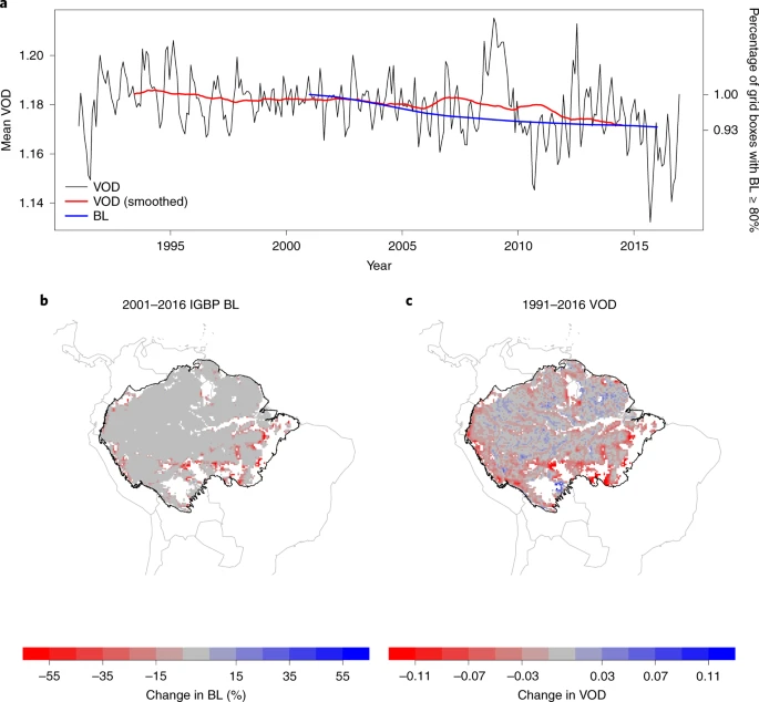
a, Time series of MODIS Land Cover evergreen BL fraction and VODCA Ku-band product. Changes in BL fraction expressed as the percentage of grid cells that have BL fraction ≥80% in each year, compared to the number of grid cells that had BL fraction ≥80% in 2001, and VOD is the monthly mean. b, Changes in the BL fraction from 2001 to 2016 for grid cells where the BL fraction is ≥80% in 2001. c, Changes in VOD from 1991 to 2016 (difference between the 2012–2016 and 1991–1995 means) for the grid cells where the BL fraction was ≥80% in 2001. Country outlines were provided by the ‘maps’ package in R and Amazon basin outline was created from http://worldmap.harvard.edu/data/geonode:amapoly_ivb (Methods).
We begin our resilience analysis by focusing on the temporal changes of AR(1), computed in sliding windows from the nonlinearly detrended and deseasonalized VOD time series (Fig. 2 and Methods). We remove forested (BL ≥ 80%) grid cells that have any human land use in them (Methods), resulting in 6,369 grid cells being analysed. The spatial distribution of the AR(1) tendency, measured by the Kendall’s rank correlation coefficient τ (Methods) at each grid cell, shows that the AR(1) increases in most of the grid cells comprising the Amazon rainforest (Fig. 2a,b). Likewise, the time series calculated from the mean AR(1) value across our study area each month shows a substantial increase over time, particularly from the early 2000s (Fig. 2c). We observe some stable or decreasing AR(1) values around the tributaries of the Amazon River, suggesting increasing resilience. VOD values can be influenced by open water but this should be minimized by looking only at grid cells where BL ≥ 80%. Previously, floodplain forests near the river, which cover 14% of the basin, have been shown to be much less resilient than the non-flooded forests throughout the Amazon39. However, when we compare grid cells in the Amazon basin floodplains and those outside (Methods), we find no significant differences between the resilience signals (Mann–Whitney U-test P = 0.579), except for a smaller Kendall τ value for floodplains from 2003 onwards (0.863 compared to 0.915; Supplementary Fig. 3).
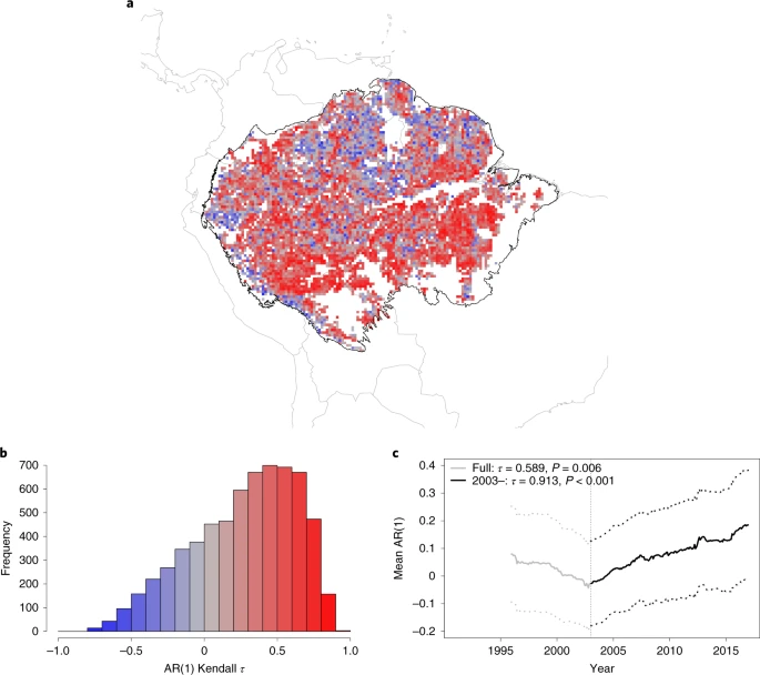
a, A map of the Kendall τ values of individual grid cells from 2003. b, Histogram of the Kendall τ values for the Amazon rainforest, considering data from 2003 onwards. Of the grid cells, 76.2% have a positive Kendall τ value from 2003 onwards and 77.8% have this for the full time series. c, Mean VOD AR(1) time series (solid line) along with ±1 s.d. (dotted lines) created from grid cells that have BL fraction ≥80% in the Amazon basin and also contain no human land use (main text and Methods). The full AR(1) time series from 1991 (grey) has a Kendall τ value of 0.589 (P = 0.006) and from 2003 (black), a value of 0.913 (P < 0.001). Note that the AR(1) values are plotted at the end of each 5-yr sliding window. Country and Amazon basin outlines produced as described in Fig. 1.
Overall, most (76.2%) of the grid cells show increasing AR(1) values from the early 2000s onwards and hence, loss of resilience (Fig. 2b), as well as 77.8% of grid cells over the full time period. Using alternative methods of detrending the VOD time series (Methods) yields similar results (Supplementary Figs. 4 and 5), as does varying the window length used to estimate AR(1) (Supplementary Fig. 6). The results are also robust to the choice of the BL fraction threshold used to determine forest, finding increasing AR(1) also when either BL ≥ 90% or BL ≥ 40% is used (Supplementary Fig. 7). Furthermore, restricting the analysis to those grid points that have BL ≥ 80% through the period 2001–2016, rather than only checking grid cells for BL ≥ 80% in 2001, shows similar signals of resilience loss (Supplementary Fig. 8). A predominance of increasing AR(1) trends is also found for the NDVI time series since 2003 (Supplementary Fig. 9).
To try and determine the causes for the detected resilience loss across the Amazon basin, we explore the relationships between the AR(1) trends and mean annual precipitation (MAP, estimated from the CHIRPS dataset40), as well as between the AR(1) trends and the distance from human land use (Methods). It has previously been suggested that drier forest is less resilient32 as well as forest nearer human land use41. We also include distance from roads alongside land use but this restricts the domain of analysis to Brazil to avoid biases by heterogeneities in road data across different countries (Supplementary Fig. 10; Methods). Figure 3 compares the spatial patterns of the AR(1) trends, MAP and human land use. Relationships with both explanatory variables are discernible, with (less common) decreases in AR(1) (Fig. 3a) being found in regions of high MAP in the north of the region (Fig. 3b) and further away from human land use (Fig. 3c). We find no confounding relationship between MAP and human land use; they are only very weakly correlated with each other (Spearman’s ρ = 0.057, P < 0.001). Hence, we can consider them as separate relationships. The computed minimum distances to human land use and roads should be interpreted as upper bounds because for the full region we do not include roads, and for the Brazil distances our dataset will not include non-federal or non-state roads, which also have human activity associated with them. Furthermore, the classification of grid cells that contain human land use at the spatial resolution used in this analysis is likely to only detect large farms and settlements.

a, VOD AR(1) Kendall τ values (as in Fig. 2a). b, MAP from the CHIRPS dataset from 1991 to 2016. c, Distance from human land use (HLU) (Methods). In a–c, MAP contours are shown, along with HLU grid cells (yellow). Supplementary Fig. 10 shows the distance from HLU or Brazilian roads for the grid cells in Brazil only. Country and Amazon basin outlines produced as described in Fig. 1.
To further explore the relationship between MAP and AR(1) trends, we create mean AR(1) time series on a moving MAP band of 500 mm (Methods). These bands show broadly the same behaviour as the region overall (Fig. 4a), with all bands showing a significant decrease in resilience post-2003 (P < 0.001 for all MAP bands). The increase in AR(1) post-2003 appears least pronounced for the highest rainfall band (3,500–4,000 mm). The strength of resilience loss increases as the MAP band decreases below 3,500–4,000 mm (Fig. 4b). For NDVI, the same relationship is also observed (Supplementary Fig. 11a,b). However, due to a large decrease in NDVI AR(1) pre-2003 across the region, analysing the full NDVI AR(1) time series yield decreasing AR(1) Kendall τ coefficients for the higher MAP bands.

a, VOD AR(1) time series for 500 mm MAP bands from 1996 (including data going back to 1991; dashed lines) and from 2003 (including data going back to 1998; solid lines). The P values of the trend significance test (Methods) are given in the legend; from 2003 onwards, they are all >0.001. b, VOD AR(1) Kendall τ series for a sliding MAP band with a width of 500 mm, from 1996 (grey) and from 2003 (black). Circles are coloured according to the corresponding time series shown in a and filled if the Kendall τ value is significantly positive (P < 0.05) and open otherwise. The tendencies of the relationships in b are τ = −0.403 (grey) and τ = −0.463 (black), confirming there is a more severe decrease in resilience with lower rainfall values. See Supplementary Fig. 15 for an uncertainty quantification of the results shown in b. The number of grid cells used to calculate the AR(1) time series and thus the Kendall τ values are shown in red in b. This never falls below 100 grid cells and so we can be confident in the mean estimation of the AR(1) time series. The number of grid cells used in the calculation of the time series in a is shown in brackets in the legend. Note that the AR(1) values are plotted at the end of each 5-yr sliding window.
To further explore the relationship between resilience and the distance to human land use, we calculate mean AR(1) time series on 50 km distance bands. Our results show that increases in AR(1) post-2003 are stronger for grid cells closer to human land use (Fig. 5a). Above 200–250 km away from human land use the signal of loss of resilience becomes less pronounced (Fig. 5b). Using the subset of Brazilian grid cells (n = 3,797) to include roads in our measurement of distance to human activity (Supplementary Fig. 10; Methods) generally reduces distances but we find a similar relationship, with decreases in Kendall τ coefficients observed up to 75 km (Fig. 5c,d). We note in both cases that, at longer distances, the number of grid cells used to calculate the AR(1) time series is lower (red lines and right-hand y axis in Fig. 5b,d). The remaining areas also tend to become more separated (the two vertical lines in Fig. 5b,d mark where <100 and <50 grid cells were left for the calculations, respectively). This helps to explain the more variable AR(1) time series at greater distances (for example, the yellow line in Fig. 5a) and the more fluctuating results for Kendall τ coefficients at greater distances (Fig. 5b,d). NDVI time series also show a loss of resilience from the early 2000s, in grid cells that are closer than 200 km from human land use (Supplementary Fig. 11c,d). We reiterate that the stated minimum distances to human land use should be viewed as upper limits with, for example, selective logging and other intrusions expected to be closer to the forest than the grid cells with major human land use and major roads. Comprehensive robustness tests, using alternative datasets and indicators, are presented in the Methods. In particular, we find overall consistent results when using the variance instead of the AR(1) as measure of resilience.

a, VOD AR(1) time series for 50 km bands measuring the minimum distance a forested grid cell is from a grid cell with human land use (defined in the Methods from the MODIS Land Cover product), from 1996 (dashed lines, these include data going back to 1991 due to the 5-yr sliding windows used to estimate the AR(1)) and from 2003 (solid lines, including data going back to 1998), with the significance of these respective tendencies shown in the legend (Methods). b, VOD AR(1) Kendall τ series for the sliding 50 km bands, from 1996 (grey, again including data going back to 1991) and from 2003 (black, including data going back to 1998). Circles are coloured according to the corresponding time series in a and are filled if the Kendall τ value is significantly positive (P < 0.05) and open otherwise. The tendencies of these relationships are τ = −0.574 (grey) and τ = −0.858 (black), showing that there is a more severe decrease in resilience with increasing proximity to human land use. The number of grid cells used to calculate the AR(1) time series and thus the Kendall τ values are shown in red in b, with vertical dotted lines denoting where there are 100 and 50 grid cells available for the calculation. The number of grid cells used in the calculation of the time series in a is shown in brackets in the legend. c,d, The same as a and b, respectively, but for the subset of grid cells in Brazil, where reliable road data are available (as shown in Supplementary Fig. 10). For this case, where the distances from any given forested grid cell to human land use or roads are computed, the trends in the Kendall τ series are τ = −0.688 and τ = −0.679, respectively.
Discussion
We reiterate that changes in the mean state of a system do not directly relate to changes in resilience. Model studies show that large parts of the Amazon rainforest can be committed to dieback16 before showing a strong change in mean state. Indeed, from our CSD indicators we infer a marked loss of Amazon rainforest resilience since the early 2000s, in vast areas where the BL fraction has not strongly decreased (compare Figs. 1b and 2a or Supplementary Fig. 8b).
Given that lower baseline MAP (Fig. 4) and greater proximity to human interference (Fig. 5) are both statistically associated with greater loss of resilience, we hypothesize that low MAP and increasing human interference could both be contributing to the large-scale loss of resilience (Fig. 2). What remains to be explained is why these two factors might play such an important role and why the large-scale resilience loss started in the early 2000s.
Previous work32 has shown that regions with lower MAP have lower absolute forest resilience, conceivably because vegetation is more water stressed and struggles to regulate its internal water content. VOD, being dependent on this water content, would consequently adjust more slowly to perturbations. Our finding that resilience has been lost faster in lower MAP regions, additionally suggests that vegetation in regions with more pronounced aridity stress is at greater risk of losing resilience. Large parts of the study region show decreasing MAP. However, the spatial pattern of MAP change (as measured by the difference between the means for January 1998 to December 2002 and January 2012 to December 2016; Supplementary Fig. 12) is different to that of AR(1) increases (Fig. 2) and we find no spatial correlation between these MAP changes and VOD AR(1) Kendall τ (Spearman’s ρ between the spatial field of MAP change and the spatial field of VOD AR(1) Kendall τ equals 0.04). Increases in dry-season length (DSL; Supplementary Fig. 12) reported in several recent studies42,43,44,45, might conceivably be a better explanatory variable but again we find no spatial correlation between DSL change and VOD AR(1) Kendall τ (ρ = −0.08). The lack of spatial correlations for both MAP and DSL could be due to the relatively short period to measure rainfall trends and for DSL due to the discrete nature of DSL values, which are given in units of full months, compared to the continuous τ values.
Despite a lack of spatial correlations, existing understanding and larger-scale aggregate measures suggest that climate variability may be among multiple factors contributing to the observed Amazon resilience loss since the early 2000s (Fig. 6). Notably, the Amazon shows signs of resilience loss during a period with three ‘one-in-a-century’ droughts10,46,47,48. Sea surface temperature (SST) anomalies in the northern tropical Atlantic Ocean (from the HadISST49 datatset; Methods) from around 2000 onwards have been generally positive compared to climatology, consistent with a shift of the Atlantic Multidecadal Oscillation (AMO) to its positive phase (Supplementary Fig. 13), although reductions in anthropogenic northern-hemisphere aerosol cooling may also play a role10. These positive northern tropical Atlantic SST anomalies led—via the associated northward shift of the Intertropical Convergence Zone—to drier conditions in the Amazon and, in particular, to two severe droughts in 2005 and 201046,48 (Fig. 6a). These two drought events are associated with corresponding peaks in the spatial-mean AR(1) time series, superimposed on the overall positive trend (see arrows in Fig. 6b). These peaks are also found in the separate AR(1) time series in Fig. 4a, appearing about 2.5 yr ahead due to the time series being plotted at the end of the 5-yr sliding windows used to calculate the AR(1) there. Moreover, a third, El Niño-driven drought in 2015/16 is accompanied by an increased overall rate of resilience loss at the very end of the time range for which the VOD data are available. The decrease in AR(1) before the early 2000s may also be linked to internal climate variability; the AMO was in its negative phase (Supplementary Fig. 13), consistent with negative SST anomalies in the northern tropical Atlantic (Fig. 6) and wetter conditions in the Amazon. The fact that the AR(1) increase since the early 2000s is statistically strongly significant suggests that it is not just due to natural climate variability.
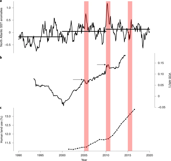
a, Northern tropical Atlantic SST anomalies averaged over 15–70° W, 5–25° N, once a mean monthly cycle has been removed. Horizontal black lines denote the decade-mean anomalies. b, Spatially averaged Amazon basin VOD AR(1) time series as in Fig. 2, plotted at the midpoint of the window used to calculate AR(1) rather than at the end of the window. c, Annual time series of percentage of grid cells in the Amazon basin that have human land use (as described in Methods). Red bands refer to 2005, 2010 and 2015, which were severe drought years in the Amazon basin. Arrows in b show the peak value in AR(1) in or near the drought years. These peak values may appear earlier due to the AR(1) time series being calculated on a moving window, compared to the SST anomalies being a monthly mean.
Increasing human land use also appears to be contributing to the observed Amazon resilience loss, with human land-use areas increasing in both reach and intensity (Fig. 6c and Supplementary Fig. 14). Notably, the expansion of human land use accelerates after 2010, in an interval that also shows accelerated resilience loss (Fig. 6b) but less striking northern tropical Atlantic SST anomalies (Fig. 6a). Greater proximity to human land use can increase disturbance factors such as direct removal of trees, construction of roads and fires, conceivably reducing absolute resilience (Fig. 5) and making the forest more prone to resilience loss.
Other factors, including rising atmospheric temperatures in response to anthropogenic greenhouse gas emissions, may additionally have negative effects on Amazon resilience (and are contributing to the warming of northern tropical Atlantic SSTs; Fig. 6a). Furthermore, the rapid change in climate is triggering ecological changes but ecosystems are having difficulties in keeping pace. In particular, the replacement of drought-sensitive tree species by drought-resistant ones is happening slower than changes in (hydro)meteorological conditions50, potentially reducing forest resilience further.
In summary, we have revealed empirical evidence that the Amazon rainforest has been losing resilience since the early 2000s, risking dieback with profound implications for biodiversity, carbon storage and climate change at a global scale. We further provided empirical evidence suggesting that overall drier conditions, culminating in three severe drought events, combined with pronounced increases in human land-use activity in the Amazon, probably played a crucial role in the observed resilience loss. The amplified loss of Amazon resilience in areas closer to human land use suggests that reducing deforestation will not just protect the parts of the forest that are directly threatened but also benefit Amazon rainforest resilience over much larger spatial scales.
Methods
Datasets
We use the Amazon basin (http://worldmap.harvard.edu/data/geonode:amapoly_ivb, accessed 28 January 2021) as our region of study. To determine the grid cells that are contained within Brazil for a subset of analysis, we use the ‘maps’ package in R (v.3.3.0; https://CRAN.R-project.org/package=maps). This is also used in the plotting of country outlines. The main dataset used to determine forest health is from VODCA33, of which we use the Ku-band product. These data are available at 0.25° × 0.25° at a monthly resolution from January 1988 to December 2016. We also use NOAA AVHRR NDVI34. For precipitation data, we use the CHIRPS dataset40 downloaded from Google Earth Engine at a monthly resolution. Finally, to determine land cover types, we used the IGBP MODIS land cover dataset MCD12C1 (ref. 37). All these datasets are at a higher spatial resolution than the VODCA dataset and thus we downscale them to match the lower resolution. Our SST data comes from HadISST49, where we define a North Atlantic region (15–70° W, 5–25° N), for which we take the spatial mean. The mean monthly cycle is then removed to produce anomalies.
For the vegetation datasets that we measure the resilience indicators on (below), we use STL decomposition (seasonal and trend decomposition using Loess)51 using the stl() function in R. This splits time series in each grid cell into an overall trend, a repeating annual cycle (by using the ‘periodic’ option for the seasonal window) and a residual component. We use the residual component in our resilience analysis. The first 3 yr of data had large jumps in VOD which were seen when testing other regions of the world as well as in the Amazon region. Hence, we restrict our analysis to the period January 1991 to December 2016.
To test the robustness of the detrending, we also vary the size of the trend window in the stl() function. The results from these alternatively detrended time series are shown in Supplementary Fig. 4. The results are also robust to varying the window used to calculate the seasonal component rather than using ‘periodic’; at the strictest plausible value of 13, we still see the same increases in AR(1) (Supplementary Fig. 5).
For the AMO index shown in Supplementary Fig. 13, data come from the Kaplan SST dataset and can be downloaded from https://psl.noaa.gov/data/timeseries/AMO/.
Grid cell selection
We use the IGBP MODIS land cover dataset at the resolution described above to determine which grid cells to use in our analysis. The dataset is available at an annual resolution from 2001 to 2018 (but we only use the time series up to 2016 to match the time span of our VOD and NDVI datasets). To focus on changes in forest resilience, we use grid cells where the evergreen BL fraction is ≥80% in 2001. Grid cells are treated as human land-use area if the built-up, croplands or vegetation mosaics fraction is >0%. We remove grid cells that have human land use in them from our forest analysis, regardless of if there is ≥80% BL fraction in the grid cell.
We measure the minimum distance between forested Amazon basin grid cells and human land-use grid cells in 2016 (believing this to be the most cautious and least biased way to measure distance) using the latitude and longitude of each grid point and computing the great-circle distance. We use human land-use grid cells over a larger area than the basin, so that we can determine the closest distance to human land use, regardless of whether this human land use lies within the basin. We also measure the minimum distance from human land use or roads in Brazil, where we have reliable data on state and federal roads (https://datacatalog.worldbank.org/dataset/brazil-road-network-federal-and-state-highways). As in the main text, we reiterate that these minimum distances can be viewed as the maximum distance from human land use as our data will not include roads for the full Amazon basin, or non-federal or non-state roads in Brazil that will have human activity associated with them.
To ensure that the pattern of changes in resilience is not a consequence of more settlements being in the southeast of the region, combined with the gradient of rainfall from northwest to southeast typical of the rainforest, we measure the correlation between MAP and the distances from the urban grid cells, which is very weak (Spearman’s ρ = 0.109, P < 0.001) and as such we are confident that there are separate processes that causes these relationships.
Resilience indicator AR(1)
We measure our resilience indicator on the residual component of the decomposed vegetation time series. We focus on AR(1), which provides a robust indicator for CSD before bifurcation-induced transitions and has been widely used for this purpose23,25,32. We measure it on a sliding window length equal to 5 yr (60 months). The sliding window creates a time series of the AR(1) coefficient in each location. Our results are robust to the sliding window length used, as shown in Supplementary Fig. 6.
From linearization and the analogy to the Ornstein–Uhlenbeck process, it holds approximately that for discrete time steps of width Δt (1 month in the case at hand):
where κ is the linear recovery rate. A decreasing recovery rate κ implies that the system’s capability to recover from perturbations is progressively lost, corresponding to diminishing stability or resilience of the attained equilibrium state. From the above equation it is clear that the AR(1) increases with decreasing κ. The point at which stability is lost and the system will undergo a critical transition to shift to a new equilibrium state, corresponds to κ = 0 and AR(1) = 1, respectively.
Measuring AR(1) across the whole time series provides information about the characteristic time scales of the two vegetation datasets we use26. Inverting κ gives the characteristic time scale of the system; for the VOD, we find 1/κ = 1.240 months, whereas for the NDVI, we find 1/κ = 0.838 months when using the mean AR(1) value across the region. This suggests that, in accordance with our interpretation of the two satellite-derived variables, the NDVI is more sensitive to shorter-term vegetation changes such as leaf greenness, while the VOD’s Ku-band is sensitive to longer-term changes such as variability in the thickness of forest stems.
Creation and tendency of AR(1) and variance time series
For analyses where either MAP bands or distance bands are used to create an AR(1) or variance series, we calculate the mean AR(1) or variance value in each month for forested (BL ≥ 80%), non-human land-use Amazon basin grid cells, from which the tendency of this mean series can be calculated. Alternatively, the Kendall τ for each band can be calculated by taking the mean Kendall τ for each individual grid cell that is within the band. Results from the first option are shown in Figs. 4 and 5 and results from the second method in Supplementary Fig. 15 for AR(1).
The tendencies of the CSD indicators are determined in terms of Kendall τ. This is a rank correlation coefficient with one variable taken to be time. Kendall τ values of 1 imply that the time series is always increasing, −1 implies that the time series is always decreasing and 0 indicates that there is no overall trend. Following previous work25,52,53, we test the statistical significance of positive tendencies using a test based on phase surrogates that preserve both the variance and the serial correlations of the time series from which the surrogates are constructed. Specifically, we compute the Fourier transform of each time series for which we want to test the significance of Kendall τ, then randomly permute the phases and finally apply the inverse Fourier transform. Since this preserves the power spectral density, it also preserves the autocorrelation function due to the Wiener–Khinchin theorem. For each time series this procedure is repeated 100,000 times to obtain the surrogates. Kendall τ is computed for each surrogate to obtain the null model distribution (corresponding to the assumption of the same variance and autocorrelation but no underlying trend), from which we calculate a P value by calculating the proportion of surrogates that have a higher Kendall τ value.
Robustness tests
To account for the possibility of human deforestation interfering with the signals we observe (which may not necessarily be detected by the MODIS Land Cover dataset) we also use the Hansen forest loss dataset54 to determine grid cells to remove in an alternate analysis. The original Hansen dataset is at a 0.00025° resolution, 1,000 times higher than the VOD dataset and as such for each VOD grid cell we measure the percentage of Hansen grid cells that show some forest loss over the time period. Note that this dataset does not specify if the observed loss is natural or caused by human deforestation. Excluding any VOD grid cells that contain more than a conservative 5% of lost forest grid cells according to this dataset and running the analysis in the main paper shows similar results. Supplementary Figs. 16–18 are recreations of Figs. 2, 4 and 5, respectively.
The loss of forest resilience observed as increasing AR(1) in both vegetation indices is supported by another indicator of CSD, namely increasing variance28—of both VOD (Supplementary Fig. 19) and NDVI (Supplementary Fig. 20). Variance is more strongly affected by changes in the frequency and amplitude of the forcing of a system and as such results could be biased towards individual events. However, we assessed the precipitation time series for changes in variance and found no relationship with the variance signals of VOD and NDVI (Supplementary Fig. 21). Nevertheless, AR(1) is considered the more robust indicator55. As another test of robustness, we partition the grid cells into those that are in floodplains and those that are not (Supplementary Fig. 3). Floodplain data are part of the NASA Large Scale Biosphere–Atmosphere Experiment (LBA-ECO)56. We also calculate the resilience signals for the C-band product of VOD for comparison (Supplementary Fig. 22). Despite the smaller temporal scale of this product, we still see increases in both AR(1) and variance. To account for a change in the number of satellites used to calculate VOD, for the Ku-band we also recreate the dataset by sampling a single random day per month rather than taking a monthly average, to mimic a constant satellite pass for the whole time period (Supplementary Fig. 23). Although this expectedly affects the absolute values of AR(1) and variance, their relative changes over time remain unaffected. To further test the robustness of our results, we looked for similar signals of resilience change in terms of trends in AR(1) in addition to variance in the precipitation time series used, as a change in the forcing could have an impact on the forest that could mistakenly be interpreted as a vegetation resilience loss. However, as for the variance, there is no clear increase in the AR(1) of precipitation, nor do the spatial patterns of both indicators reveal any relationship between changing precipitation AR(1) and variance and the observed vegetation resilience loss. Hence, we are confident that changes in precipitation forcing are not driving the vegetation AR(1) signals.
Data availability
The VOD dataset is available from https://zenodo.org/record/2575599#.YHRE6RRKj7E. The NDVI dataset is available from https://www.ncei.noaa.gov/metadata/geoportal/rest/metadata/item/gov.noaa.ncdc:C01558/html. The MODIS Land Cover dataset is available from https://lpdaac.usgs.gov/products/mcd12c1v006. The CHIRPS precipitation dataset is available from https://data.chc.ucsb.edu/products/CHIRPS-2.0/global_2-monthly/tifs. The Amazon basin shapefile is available from http://worldmap.harvard.edu/data/geonode:amapoly_ivb. Brazilian road data are available from https://datacatalog.worldbank.org/dataset/brazil-road-network-federal-and-state-highways. SST data from HadISST are available from https://www.metoffice.gov.uk/hadobs/hadisst/.
Code availability
All data and code used for the analysis are available on request from the corresponding author and are published online57.
References
Lenton, T. M. et al. Tipping elements in the Earth’s climate system. Proc. Natl Acad. Sci. USA 105, 1786–1793 (2008).
Dirzo, R. & Raven, P. H. Global state of biodiversity and loss. Ann. Rev. Environ. Res. 28, 137–167 (2003).
Malhi, Y. et al. Climate change, deforestation, and the fate of the Amazon. Science 319, 169–172 (2008).
Gatti, L. V. et al. Amazonia as a carbon source linked to deforestation and climate change. Nature 595, 388–393 (2021).
Brienen, R. J. W. et al. Long-term decline of the Amazon carbon sink. Nature 519, 344–348 (2015).
Feldpausch, T. R. et al. Amazon forest response to repeated droughts. Glob. Biogeochem. Cycles 30, 964–982 (2016).
Hubau, W. et al. Asynchronous carbon sink saturation in African and Amazonian tropical forests. Nature 579, 80–87 (2020).
Boers, N., Marwan, N., Barbosa, H. M. J. & Kurths, J. A deforestation-induced tipping point for the South American monsoon system. Sci. Rep. 7, 41489 (2017).
Cox, P. M., Betts, R. A., Jones, C. D., Spall, S. A. & Totterdell, I. J. Acceleration of global warming due to carbon-cycle feedbacks in a coupled climate model. Nature 408, 184–187 (2000).
Cox, P. M. et al. Increasing risk of Amazonian drought due to decreasing aerosol pollution. Nature 453, 212–215 (2008).
Lovejoy, T. E. & Nobre, C. Amazon tipping point. Sci. Adv. 4, eaat2340 (2018).
Lovejoy, T. E. & Nobre, C. Amazon tipping point: last chance for action. Sci. Adv. 5, eaba2949 (2019).
Brando, P. M. et al. Abrupt increases in Amazonian tree mortality due to drought–fire interactions. Proc. Natl Acad. Sci. USA 111, 6347–6352 (2014).
Pueyo, S. et al. Testing for criticality in ecosystem dynamics: the case of Amazonian rainforest and savanna fire. Ecol. Lett. 13, 793–802 (2010).
Salati, E., Dall’Olio, A., Matsui, E. & Gat, J. R. Recycling of water in the Amazon basin: an isotopic study. Water Resour. Res. 15, 1250–1258 (1979).
Jones, C., Lowe, J., Liddicoat, S. & Betts, R. Committed terrestrial ecosystem changes due to climate change. Nat. Geosci. 2, 484–487 (2009).
Boulton, C. A., Booth, B. B. B. & Good, P. Exploring uncertainty of Amazon dieback in a perturbed parameter Earth system ensemble. Glob. Change Biol. 23, 5032–5044 (2017).
Huntingford, C. et al. Simulated resilience of tropical rainforests to CO2-induced climate change. Nat. Geosci. 6, 268–273 (2013).
Friend, A. D., Stevens, A. K., Knox, R. G. & Cannell, M. G. R. A process-based, terrestrial biosphere model of ecosystem dynamics (Hybrid v3.0). Ecol. Model. 95, 249–287 (1997).
Poulter, B. et al. Robust dynamics of Amazon dieback to climate change with perturbed ecosystem model parameters. Glob. Change Biol. 16, 2476–2495 (2010).
Sitch, S. et al. Evaluation of the terrestrial carbon cycle, future plant geography and climate-carbon cycle feedbacks using five Dynamic Global Vegetation Models (DGVMs). Glob. Change Biol. 14, 2015–2039 (2008).
Wissel, C. A universal law of the characteristic return time near thresholds. Oecologia 65, 101–107 (1984).
Scheffer, M. et al. Early-warning signals for critical transitions. Nature 461, 53–59 (2009).
Pimm, S. L. The complexity and stability of ecosystems. Nature 307, 321–326 (1984).
Dakos, V. et al. Slowing down as an early warning signal for abrupt climate change. Proc. Natl Acad. Sci. USA 105, 14308–14312 (2008).
Held, H. & Kleinen, T. Detection of climate system bifurcations by degenerate fingerprinting. Geophys. Res. Lett. https://doi.org/10.1029/2004gl020972 (2004).
Boulton, C. A., Good, P. & Lenton, T. M. Early warning signals of simulated Amazon rainforest dieback. Theor. Ecol. 6, 373–384 (2013).
Lenton, T. M. Early warning of climate tipping points. Nat. Clim. Change 1, 201–209 (2011).
Biggs, R., Carpenter, S. R. & Brock, W. A. Turning back from the brink: detecting an impending regime shift in time to avert it. Proc. Natl Acad. Sci. USA 106, 826–831 (2009).
Boers, N. & Rypdal, M. Critical slowing down suggests that the western Greenland Ice Sheet is close to a tipping point. Proc. Natl Acad. Sci. USA 118, e2024192118 (2021).
Boers, N. Observation-based early-warning signals for a collapse of the Atlantic Meridional Overturning Circulation. Nat. Clim. Change 11, 680–688 (2021).
Verbesselt, J. et al. Remotely sensed resilience of tropical forests. Nat. Clim. Change 6, 1028–1031 (2016).
Moesinger, L. et al. The global long-term microwave Vegetation Optical Depth Climate Archive (VODCA). Earth Syst. Sci. Data 12, 177–196 (2020).
NOAA Climate Data Record (CDR) of AVHRR Normalized Difference Vegetation Index (NDVI), Version 5 (NOAA National Centers for Environmental Information, accessed 10 February 2021); https://doi.org/10.7289/V5ZG6QH9
Liu, Y. Y. et al. Recent reversal in loss of global terrestrial biomass. Nat. Clim. Change 5, 470–474 (2015).
Myneni, R. B., Keeling, C. D., Tucker, C. J., Asrar, G. & Nemani, R. R. Increased plant growth in the northern high latitudes from 1981 to 1991. Nature 386, 698–702 (1997).
Friedl, M. & Sulla-Menashe, D. MCD12C1, Version 6 (NASA EOSDIS Land Processes DAAC, accessed 20 April 2020); https://doi.org/10.5067/MODIS/MCD12C1.006
Tian, F. et al. Remote sensing of vegetation dynamics in drylands: evaluating vegetation optical depth (VOD) using AVHRR NDVI and in situ green biomass data over West African Sahel. Remote Sens. Environ. 177, 265–276 (2016).
Flores, B. M. et al. Floodplains as an Achilles’ heel of Amazonian forest resilience. Proc. Natl Acad. Sci. USA 114, 4442–4446 (2017).
Funk, C. et al. The climate hazards infrared precipitation with stations—a new environmental record for monitoring extremes. Sci. Data 2, 150066 (2015).
Wuyts, B., Champneys, A. R. & House, J. I. Amazonian forest–savanna bistability and human impact. Nat. Commun. 8, 15519 (2017).
Fu, R. et al. Increased dry-season length over southern Amazonia in recent decades and its implication for future climate projection. Proc. Natl Acad. Sci. USA 110, 18110–18115 (2013).
Marengo, J. A. et al. Changes in climate and land use over the Amazon region: current and future variability and trends. Front. Earth Sci. https://doi.org/10.3389/feart.2018.00228 (2018).
Leite-Filho, A. T., Sousa Pontes, V. Y. & Costa, M. H. Effects of deforestation on the onset of the rainy season and the duration of dry spells in southern Amazonia. J. Geophys. Res. Atmos. 124, 5268–5281 (2019).
Leite‐Filho, A. T., Costa, M. H. & Fu, R. The southern Amazon rainy season: the role of deforestation and its interactions with large‐scale mechanisms. Int. J. Climatol. https://doi.org/10.1002/joc.6335 (2019).
Lewis, S. L., Brando, P. M., Phillips, O. L., Van Der Heijden, G. M. F. & Nepstad, D. The 2010 Amazon drought. Science 331, 554 (2011).
Erfanian, A., Wang, G. & Fomenko, L. Unprecedented drought over tropical South America in 2016: significantly under-predicted by tropical SST. Sci. Rep. 7, 5811 (2017).
Ciemer, C. et al. An early-warning indicator for Amazon droughts exclusively based on tropical Atlantic sea surface temperatures. Environ. Res. Lett. 15, 094087 (2020).
Rayner, N. A. et al. Global analyses of sea surface temperature, sea ice, and night marine air temperature since the late nineteenth century. J. Geophys. Res. https://doi.org/10.1029/2002jd002670 (2003).
Esquivel‐Muelbert, A. et al. Compositional response of Amazon forests to climate change. Glob. Change Biol. 25, 39–56 (2019).
Cleveland, R. B., Cleveland, W. S. & Terpenning, I. STL: a seasonal-trend decomposition procedure based on Loess. J. Off. Stat. 6, 3 (1990).
Rypdal, M. Early-warning signals for the onsets of Greenland interstadials and the younger dryas–preboreal transition. J. Clim. 29, 4047–4056 (2016).
Boers, N. Early-warning signals for Dansgaard–Oeschger events in a high-resolution ice core record. Nat. Commun. 9, 2556 (2018).
Hansen, M. C. et al. High-resolution global maps of 21st-century forest cover change. Science 342, 850–853 (2013).
Dakos, V., Van Nes, E. H., D’Odorico, P. & Scheffer, M. Robustness of variance and autocorrelation as indicators of critical slowing down. Ecology 93, 264–271 (2012).
Hess, L. L. et al. LBA-ECO LC-07 Wetland Extent, Vegetation, and Inundation: Lowland Amazon Basin (ORNL DAAC, 2005); https://doi.org/10.3334/ORNLDAAC/1284
Boulton, C. A. Amazon rainforest resilience data. Zenodo https://doi.org/10.5281/zenodo.5837469 (2022).
Acknowledgements
We thank B. Sakschewski for his helpful comments on the research. N.B. acknowledges funding by the Volkswagen Foundation. This is TiPES contribution no. 107. The TiPES project (‘Tipping Points in the Earth System’) has received funding from the European Union’s Horizon 2020 research and innovation programme under grant agreement no. 820970. C.A.B. and T.M.L. were supported by the Leverhulme Trust (RPG-2018-046). T.M.L. was also supported by a grant from The Alan Turing Institute under a Turing Fellowship (R-EXE-001).
Author information
Authors and Affiliations
Contributions
N.B. and C.A.B. conceived and designed the study with input from T.M.L. C.A.B. performed the numerical analysis with contributions from N.B. All authors discussed and interpreted results, drew conclusions and wrote the paper.
Corresponding author
Ethics declarations
Competing interests
The authors declare no competing interests.
Peer review
Peer review information
Nature Climate Change thanks Albertus J. Dolman, Bernardo Flores and the other, anonymous, reviewer(s) for their contribution to the peer review of this work.
Additional information
Publisher’s note Springer Nature remains neutral with regard to jurisdictional claims in published maps and institutional affiliations.
Supplementary information
Supplementary Information
Supplementary Figs. 1–23.
Rights and permissions
Open Access This article is licensed under a Creative Commons Attribution 4.0 International License, which permits use, sharing, adaptation, distribution and reproduction in any medium or format, as long as you give appropriate credit to the original author(s) and the source, provide a link to the Creative Commons license, and indicate if changes were made. The images or other third party material in this article are included in the article’s Creative Commons license, unless indicated otherwise in a credit line to the material. If material is not included in the article’s Creative Commons license and your intended use is not permitted by statutory regulation or exceeds the permitted use, you will need to obtain permission directly from the copyright holder. To view a copy of this license, visit http://creativecommons.org/licenses/by/4.0/.
About this article

Cite this article
Boulton, C.A., Lenton, T.M. & Boers, N. Pronounced loss of Amazon rainforest resilience since the early 2000s. Nat. Clim. Chang. 12, 271–278 (2022). https://doi.org/10.1038/s41558-022-01287-8
Received:
Accepted:
Published:
Issue Date:
DOI: https://doi.org/10.1038/s41558-022-01287-8
This article is cited by
-
Amazon savannization and climate change are projected to increase dry season length and temperature extremes over Brazil
Scientific Reports (2024)
-
Remotely sensing potential climate change tipping points across scales
Nature Communications (2024)
-
Protecting Life and Lung: Protected Areas Affect Fine Particulate Matter and Respiratory Hospitalizations in the Brazilian Amazon Biome
Environmental and Resource Economics (2024)
-
Assessing inconsistencies in historical land-use reconstructions for Africa at 1800
Regional Environmental Change (2024)
-
Accessing the specialized metabolome of actinobacteria from the bulk soil of Paullinia cupana Mart. on the Brazilian Amazon: a promising source of bioactive compounds against soybean phytopathogens
Brazilian Journal of Microbiology (2024)
