Engineering fast high-fidelity quantum operations with constrained interactions

Abstract

Understanding how to tailor quantum dynamics to achieve the desired evolution is a crucial problem in almost all quantum technologies. Oftentimes an otherwise ideal quantum dynamics is corrupted by unavoidable interactions, and finding ways to mitigate the unwanted effects of such interactions on the dynamics is a very active field of research. Here, we present a very general method for designing high-efficiency control sequences that are fully compatible with experimental constraints on available interactions and their tunability. Our approach relies on the Magnus expansion to find order by order the necessary corrections that result in a high-fidelity operation. In the end finding, the control fields are reduced to solve a set of linear equations. We illustrate our method by applying it to a number of physically relevant problems: the strong-driving limit of a two-level system, fast squeezing in a parametrically driven cavity, the leakage problem in transmon qubit gates, and the acceleration of SNAP gates in a qubit-cavity system.

Introduction

The success of any nascent quantum technology will ultimately be limited by our ability to manipulate relevant quantum states. Finding the required time-dependent control fields that generate with high accuracy a desired unitary evolution is in general not a trivial task: it is sufficient to consider a simple driven two-level system in the strong-driving limit^1,2,3 to find an example of a complex control problem. This generic problem becomes even more complicated when including realistic constraints: unavailable control fields, bandwidth, and amplitude limitations, etc. Finding widely applicable methods to attack such problems is thus highly desirable.

There are of course many existing approaches to quantum control. Of these, the most ubiquitous is to exploit numerical algorithms (see refs. ^4,5,6,7,8,9) based on optimal quantum control theory¹⁰. The methods ultimately rely on the numerical optimization of an objective function, for example, the fidelity of a desired target state with the actual time-evolved state. For many problems, the effective landscape of the objective function has many local minima, which can make it challenging to find the truly optimal protocol. While methods to overcome these limitations exist^11,12,13,14, they become difficult to implement as the dimension of the control space increases. An alternative approach is to use an analytical method to design effective protocols; control pulses designed in this way could then be further improved by using them to seed a numerical optimal control algorithm. Analytic methods are, however, often system-specific (see refs. ^15,16), or only work with a specific restricted class of dynamics (e.g., methods based on shortcuts to adiabaticity, which are specific to protocols based on adiabatic evolution^{17,18,19,20,21,22,23}). These approaches are also generally impractical in systems with many degrees of freedom or sufficiently complex interactions.

In this work, we present a general framework for constructing control fields that realize the desired evolution, in a manner that is explicitly consistent with experimental constraints. At its heart, it allows one to use the analytic solution of a simple control problem to then find a high-fidelity pulse sequence for a more complex problem where a closed-form analytic solution is not possible. Our method has many potential virtues: it is applicable to an extremely wide class of systems and protocols, produces smooth control fields, and only requires one to numerically solve a finite set of linear equations. It builds on the recently proposed Magnus-based control method introduced in ref. ²⁴ but greatly extends its power and applicability.

Our generic goal is to use a specific time-dependent Hamiltonian $\hat{H}(t)$ (whose form and tunability are constrained) to produce (at time t_f) a desired unitary operation. We start by splitting the Hamiltonian into two parts as $\hat{H}(t)={\hat{H}}_{0}(t)+\hat{V}(t)$, where H₀(t) is simple enough to be analytically tractable, and $\hat{V}(t)$ represents all the additional interactions that make the problem unsolvable. The basic strategy then has two parts:

• (1) First, choose control fields in the "simple" Hamiltonian ${\hat{H}}_{0}(t)$ so that in the absence of $\hat{V}(t)$, one realizes the desired operation. This can be done analytically.

• (2) Adding back $\hat{V}(t)$ will then destroy the ideal evolution. We address this by modifying available control fields so as to average out the impact of $\hat{V}(t)$. This amounts to adding a control correction to the full Hamiltonian: $\hat{H}(t)\to \hat{H}(t)+\hat{W}(t)$ (see Fig. 1a).

  Fig. 1: Generic quantum control problem.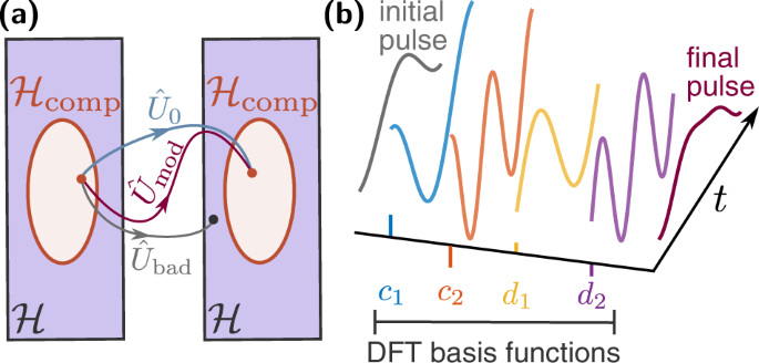

  

  a An idealized unitary evolution (${\hat{U}}_{0}$) maps an initial quantum state into a desired final state. The real evolution ($\hat{U}$) does not allow one to reach the desired final state because it gets spoil by unwanted interactions neglected when deriving ${\hat{U}}_{0}$. The effects of these interactions can be made arbitrary small by modifying the idealized control fields (${\hat{U}}_{{\rm{mod}}}$). b The idealized control fields are modified by adding a finite number of basis functions, e.g., discrete Fourier transform (DFT) basis functions, multiplied by free weights. The free weights are chosen such that the final pulse averages away the effects of the unwanted interactions.

The question is of course how to find the desired control correction $\hat{W}(t)$. We address this using the strategy described recently in ref. ²⁴, where $\hat{W}(t)$ is found perturbatively using a Magnus expansion^25,26. A major limitation of this approach is that it often requires terms in $\hat{W}(t)$ that are incompatible with the physical system at hand (e.g., interaction terms that do not exist, or that cannot be made time-dependent in the given experimental platform). This is where this work makes a substantial contribution. We introduce a way to find terms in the series expansion of $\hat{W}(t)$ that are always compatible with all constraints. We achieve this by expanding $\hat{W}(t)$ at each order as a finite sum of time-dependent basis functions multiplied by free weights. Finding the required control corrections then amounts in most cases to solving time-independent linear equations for these weights.

As we demonstrate through several examples, this methodology is both extremely flexible and effective; it can also work in systems with many degrees of freedom. The examples we consider in “Results” include the strong non-RWA driving of a qubit, leakage errors in a superconducting qubit, rapid squeezing generation in a parametrically driven bosonic mode, and accelerated SNAP gates^27,28 in a coupled transmon-cavity system.

Note that the general idea of looking for control fields represented as a finite combination of basis functions was previously used in refs. ^29,30 to design two-qubit superconducting qubit gates that minimize leakage errors. In contrast to those works, our work is both more general and more systematic. Our approach is also complementary to a variational approach for approximately finding shortcuts-to-adiabaticity protocols in complex systems that are compatible with experimental constraints^31,32.

Results

Imperfect unitary evolution

We consider the generic Hamiltonian:

$$\hat{H}(t)={\hat{H}}_{0}(t)+\epsilon \hat{V}(t).$$

(1)

The Hamiltonian ${\hat{H}}_{0}(t)$ generates the desired time evolution, while $\hat{V}(t)$ is the spurious “error” Hamiltonian that disrupts the ideal dynamics and which can be treated as a perturbation. The perturbative character of $\hat{V}(t)$ can originate, e.g., from $\hat{V}(t)$ being proportional to a parameter ϵ ≪ 1, or because $\hat{V}(t)$ is a fast oscillating function. In Supplementary Note 1, we show why nonresonant error-Hamiltonians can also be corrected with the method presented below. In this section, however, we consider the situation where $\hat{V}(t)$ is proportional to a parameter ϵ ≪ 1 simply because this allows one to count the orders of the perturbative series in a straightforward way. We stress, however, that one can apply the method that we are about to introduce independently of the reason that makes $\hat{V}(t)$ a perturbation.

The time evolution operator generated by $\hat{H}(t)$ is given by

$$\hat{U}(t)={\hat{U}}_{0}(t){\hat{U}}_{{\rm{I}}}(t).$$

(2)

Here, ${\hat{U}}_{0}(t)$ represents the ideal time evolution generated by ${\hat{H}}_{0}(t)$ (ℏ = 1),

$${\hat{U}}_{0}(t)=\hat{T}\exp \left[-{\rm{i}}\mathop{\int}\nolimits_{\!0}^{t}\ {\rm{d}}{t}_{1}{\hat{H}}_{0}({t}_{1})\right],$$

(3)

where $\hat{T}$ is the time-ordering operator, and we assume that the time evolution starts at t = 0. The effect of the error Hamiltonian $\hat{V}(t)$ on the dynamics is given by ${\hat{U}}_{{\rm{I}}}(t)$, which is defined as

$${\hat{U}}_{{\rm{I}}}(t)=\hat{T}\exp \left[-{\rm{i}}\epsilon \mathop{\int}\nolimits_{\!0}^{t}\ {\rm{d}}{t}_{1}{\hat{V}}_{{\rm{I}}}({t}_{1})\right].$$

(4)

Here, an operator $\hat{O}(t)$ in the interaction picture is given by ${\hat{O}}_{{\rm{I}}}(t)={\hat{U}}_{0}^{\dagger }(t)\hat{O}(t){\hat{U}}_{0}(t)$.

Our goal is to have the time evolution operator at t = t_f match a specific desired unitary operator ${\hat{U}}_{{\rm{G}}}$; the form of the time evolution operator at earlier times is not relevant for us. This is the case in many problems, the most prominent example being the engineering of quantum gates. We also assume that ${\hat{H}}_{0}(t)$ provides us the desired time evolution at t = t_f, i.e., ${\hat{U}}_{0}({t}_{{\rm{f}}})={\hat{U}}_{{\rm{G}}}$. Consequently, the presence of a nonzero error Hamiltonian $\hat{V}(t)$ disrupts the evolution and prevents us to generate the desired evolution, since in general ${\hat{U}}_{{\rm{I}}}({t}_{{\rm{f}}})\,\ne \,{\mathbb{1}}$ (see Eq. (2)).

General strategy to correct unitary evolution

To obtain the ideal unitary evolution at t = t_f, we wish to modify the time dependence of $\hat{H}(t)$ to cancel the deleterious effects of $\hat{V}(t)$. This is formally accomplished by introducing the modified Hamiltonian

$${\hat{H}}_{{\rm{mod}}}(t)={\hat{H}}_{0}(t)+\epsilon \hat{V}(t)+\hat{W}(t).$$

(5)

Here, $\hat{W}(t)$ is an unknown control Hamiltonian that cancels, or at least mitigates, the effects of $\hat{V}(t)$ on the dynamics, bringing us closer to the desired time evolution (see Fig. 1a). The unitary evolution generated by ${\hat{H}}_{{\rm{mod}}}(t)$ is given by ${\hat{U}}_{{\rm{mod}}}(t)={\hat{U}}_{0}(t){\hat{U}}_{{\rm{mod}},{\rm{I}}}(t)$, where

$${\hat{U}}_{{\rm{mod}},{\rm{I}}}(t)=\hat{T}\exp \left[-{\rm{i}}\mathop{\int}\nolimits_{\!0}^{t}\ {\rm{d}}{t}_{1}{\hat{H}}_{{\rm{mod}},{\rm{I}}}({t}_{1})\right]$$

(6)

is the unitary evolution operator generated by

$${\hat{H}}_{{\rm{mod}},{\rm{I}}}(t)=\epsilon {\hat{V}}_{{\rm{I}}}(t)+{\hat{W}}_{{\rm{I}}}(t),$$

(7)

the modified Hamiltonian in the interaction picture with respect to ${\hat{H}}_{0}(t)$. The desired unitary operator at t = t_f is achieved if ${\hat{U}}_{{\rm{mod}},{\rm{I}}}({t}_{{\rm{f}}})={\mathbb{1}}$, i.e., ${\hat{U}}_{{\rm{mod}}}({t}_{{\rm{f}}})={\hat{U}}_{0}({t}_{{\rm{f}}})={\hat{U}}_{{\rm{G}}}$.

A trivial solution to this problem is to take $\hat{W}(t)=-\epsilon \hat{V}(t)$. This solution is almost always infeasible, as the general form of $\hat{W}(t)$ will be constrained by the kinds of interactions available in the system and their tunability. Furthermore, we are only interested in generating the correct unitary at t = t_f and consequently canceling the spurious Hamiltonian at all times is in some sense demanding more than it is required. A better solution consists of canceling the spurious Hamiltonian on average, where one makes use of the fact that the time evolution at intermediate times is not important. This idea has been used early on to address the problem of population inversion in magnetic nuclear resonance^33,34. Here, we choose to exploit this idea by following the procedure introduced in ref. ²⁴. This leads to relatively lax conditions that the control Hamiltonian $\hat{W}(t)$ must satisfy. Nevertheless, finding an exact $\hat{W}(t)$ is a complex task and generally one needs to resort to perturbation theory to find approximated solutions.

Let us start by writing $\hat{W}(t)$ as a series in ϵ,

$$\hat{W}(t)=\mathop{\sum }\limits_{n=1}^{\infty }{\epsilon }^{n}{\hat{W}}^{(n)}(t).$$

(8)

In order to find $\hat{W}(t)$, one could work with the series expansion of the time-ordered exponential of Eq. (6), but a more convenient approach is to use the Magnus expansion^25,26. With the Magnus expansion we can convert the complicated time-ordered exponential to a simple exponential of an operator that can be expanded in a series:

$${\hat{U}}_{{\rm{mod}},{\rm{I}}}(t)=\exp \left[\mathop{\sum }\limits_{l=1}^{\infty }{\hat{{{\Omega }}}}_{l}(t)\right].$$

(9)

The terms of the Magnus expansion, ${\hat{{{\Omega }}}}_{l}(t)$, are recursively defined by differential equations^25,26, with the first two terms being given by

$${\partial }_{t}{\hat{{{\Omega }}}}_{1}(t)=-{\rm{i}}{\hat{H}}_{{\rm{mod}},{\rm{I}}}(t),$$

(10)

$${\partial }_{t}{\hat{{{\Omega }}}}_{2}(t)=\frac{1}{2}[{\partial }_{t}{\hat{{{\Omega }}}}_{1}(t),{\hat{{{\Omega }}}}_{1}(t)].$$

(11)

In order to correct the dynamics up to order ${\mathcal{O}}({\epsilon }^{m})$, one needs to find a control Hamiltonian $\hat{W}(t)$ such that ${\hat{{{\Omega }}}}_{l}({t}_{{\rm{f}}})={\bf{0}}$ for l = 1, …, m. As shown in ref. ²⁴, this is accomplished if one firstly truncates the series representing $\hat{W}(t)$ (see Eq. (8)) up to order m and then requires the operators ${\hat{W}}_{{\rm{I}}}^{(n)}(t)$, for n = 1, …, m, to satisfy the following equation:

$${\epsilon }^{n}\mathop{\int}\nolimits_{\!0}^{{t}_{{\rm{f}}}}\ {\rm{d}}t\,{\hat{W}}_{{\rm{I}}}^{(n)}(t)=-{\rm{i}}\mathop{\sum }\limits_{l = 1}^{n}{\hat{{{\Omega }}}}_{l}^{(n-1)}({t}_{{\rm{f}}}).$$

(12)

Here, ${\hat{{{\Omega }}}}_{l}^{(n)}(t)$ is the lth term of the Magnus expansion associated with the partially corrected Hamiltonian

$${\hat{H}}_{{\rm{mod}},{\rm{I}}}^{(n)}(t)=\epsilon {\hat{V}}_{{\rm{I}}}(t)+\mathop{\sum }\limits_{l = 1}^{n}{\epsilon }^{l}{\hat{W}}_{{\rm{I}}}^{(l)}(t).$$

(13)

Note that in Eq. (13), the series representing the correction $\hat{W}(t)$ has been truncated at order n. To first order (m = 1), Eq. (12) reduces to

$$\mathop{\int}\nolimits_{\!0}^{{t}_{{\rm{f}}}}\ {\rm{d}}t\,{\hat{W}}_{{\rm{I}}}^{(1)}(t)=-\mathop{\int}\nolimits_{\!0}^{{t}_{{\rm{f}}}}\ {\rm{d}}t\,{\hat{V}}_{{\rm{I}}}(t).$$

(14)

Equation (12) is the only restriction on the terms of the control Hamiltonian $\hat{W}(t)$. This implies we have considerable latitude in how we make our specific choice of $\hat{W}(t)$. In what follows, we fully exploit this freedom to systematically find control Hamiltonians that are completely compatible with experimental constraints on kinds and tunability of available interactions.

Constrained control Hamiltonians

To proceed, we introduce a set of N_op time-independent Hermitian operators $\{{\hat{A}}_{j}\}$ that form a basis for ${\hat{H}}_{0}(t)$, $\hat{V}(t)$, and $\hat{W}(t)$. By this, we mean that these operators allow for a unique decomposition of the different Hamiltonian operators at each instant of time:

$${\hat{H}}_{0}(t)=\sum _{j}{h}_{j}(t){\hat{A}}_{j},$$

(15)

$$\hat{V}(t)=\sum _{j}{v}_{j}(t){\hat{A}}_{j},$$

(16)

$${\hat{W}}^{(n)}(t)=\sum _{j}{w}_{j}^{(n)}(t){\hat{A}}_{j}.$$

(17)

Here, h_j(t), v_j(t), and ${w}_{j}^{(n)}(t)$ are the real control fields (expansion coefficients) associated with the decomposition of ${\hat{H}}_{0}(t)$, $\hat{V}(t)$, and ${\hat{W}}^{(n)}(t)$, respectively. For instance, the elements of the set $\{{\hat{A}}_{j}\}$ for a two-level system are the Pauli operators ${\hat{\sigma }}_{j}$ with j ∈ {1, 3}. We also introduce the Lie algebra ${\mathfrak{g}}$ generated by the set of operators $\{-{\rm{i}}{\hat{A}}_{j}\}$ with the Lie bracket given by the commutation operation. Having a Lie algebra ensures that one can use the basis formed by the set $\{{\hat{A}}_{j}\}$ to decompose the operators generated by the Magnus expansion. Finally, we stress that N_op can be finite even if the dimension of the Hilbert space is infinite. This is the case for quadratic bosonic forms that can be characterized by the special unitary groups SU(2) or SU(1, 1), which are associated with the Lie algebras su(2) or su(1, 1)³⁵.

Transforming Eqs. (16) and (17) to the interaction picture defined by ${\hat{H}}_{0}(t)$, we have

$${\hat{V}}_{{\rm{I}}}(t)=\sum _{j}{v}_{j}(t){\hat{A}}_{j,{\rm{I}}} (t).$$

(18)

Using the fact that $\{{\hat{A}}_{j}\}$ forms a basis, we can write

$${\hat{A}}_{j,{\rm{I}}} (t) =\sum _{l}{a}_{jl}(t){\hat{A}}_{l}.$$

(19)

Here, the functions a_jl(t) fully encode the action of the interaction picture transformation on our basis operators.

Substituting Eq. (19) in Eq. (18), we obtain

$${\hat{V}}_{{\rm{I}}}(t)=\sum _{j}{\tilde{v}}_{j}(t){\hat{A}}_{j},$$

(20)

where we use tildes to denote control fields in the interaction picture, and we have

$${\tilde{v}}_{j}(t)=\sum _{l}{a}_{lj}(t){v}_{l}(t).$$

(21)

Proceeding analogously for ${\hat{W}}^{(n)}(t)$ we get

$${\hat{W}}_{{\rm{I}}}^{(n)}(t)=\sum _{j}{\tilde{w}}_{j}^{(n)}(t){\hat{A}}_{j},$$

(22)

with

$${\tilde{w}}_{j}^{(n)}(t)=\sum _{l}{a}_{lj}(t){w}_{l}^{(n)}(t).$$

(23)

We now return to the fundamental equations of our approach, Eqs. (12), which need to be satisfied to cancel the effects of $\hat{V}(t)$ to the desired order. As written, these equations do not reflect any information about relevant experimental constraints. Typical examples of constraints are the inability to control the fields that couple to certain ${\hat{A}}_{j}$, i.e., that particular field has to obey ${w}_{j}^{(n)}(t)=0$. Note that in general, it is possible to have h_j(t) ≠ 0 while one must work with the condition ${w}_{j}^{(n)}(t)=0$. Moreover, even if ${w}_{j}^{(n)}(t)$ can be controlled, it might have restrictions, e.g., ${w}_{j}^{(n)}(t)$ must be time-independent or it has bandwidth limitations. In the following, we show how to derive equations for ${w}_{j}^{(n)}(t)$ that obey Eq. (12) and simultaneously fulfill the previously mentioned constraints. This then enables the design of high-fidelity control pulses that are fully compatible with experimental constraints. As we discuss below, it is enough to show how one derives equations for the first-order control fields ${w}_{j}^{(1)}(t)$, which must obey Eq. (14), since the procedure for ${w}_{j}^{(n)}(t)$ is similar.

We proceed by substituting Eqs. (20) and (22) into Eq. (14), which determines the first-order correction Hamiltonian. We obtain an operator equation which can be split into N_op equations, one for each operator ${\hat{A}}_{j}$:

$$\mathop{\int}\nolimits_{\!0}^{{t}_{{\rm{f}}}}\ {\rm{d}}t{\tilde{w}}_{j}^{(1)}(t)=-\mathop{\int}\nolimits_{\!0}^{{t}_{{\rm{f}}}}\ {\rm{d}}t{\tilde{v}}_{j}(t).$$

(24)

We stress that it is possible to have ${\tilde{w}}_{j}^{(1)}(t)\,=\,0$ while ${\tilde{v}}_{j}(t)\,\ne\,0$ for certain values of j. We call a correction Hamiltonian with such limitations singular since Eq. (24) cannot be solved for every j. We show in the subsection “The Magnus Correction for Singular or Ill-conditioned Correction Hamiltonians” of “Results” that one can still use a singular correction Hamiltonian to cancel all unwanted interactions generated by $\hat{V}(t)$, but for now we focus on the simpler case of non-singular correction Hamiltonians.

The problem still remains of how to solve for ${w}_{j}^{(1)}(t)$; this is still a complex task since one is dealing with a system of N_op coupled integral equations. This problem can be overcome by choosing an appropriate parametrization for the functions ${w}_{j}^{(1)}(t)$. Here, since ${w}_{j}^{(1)}(t)$ must only have support on the interval [0, t_f], we use a finite Fourier series decomposition,

$${w}_{j}^{(1)}(t)=\mathop{\sum }\limits_{k=0}^{{k}_{\max ,j}}{c}_{jk}^{(1)}\cos \left({\omega }_{k}t\right)+{d}_{jk}^{(1)}\sin \left({\omega }_{k}t\right),$$

(25)

with ω_k = 2πk/t_f and ${d}_{j0}^{(1)}=0$. This parametrization allows us to carry out the time integration over the duration of the protocol and use the Fourier coefficients as the free parameters to satisfy the system of equations given by Eq. (24). We stress that at this stage finding the first-order correction that fulfills Eq. (14) has been reduced to determining a set of ${N}_{{\rm{coeffs}}}=\mathop{\sum }\nolimits_{j = 1}^{{N}_{{\rm{op}}}}(2{k}_{\max ,j}+1)$ coefficients. Note that one could use other basis functions for the decomposition, e.g., Slepian functions^36,37,38. We remind the reader that we performed three series expansions up to now: the perturbative expansion, for which we use the super-index (n) (in Eq. (25) n = 1), the operator expansion in the $\{{\hat{A}}_{j}\}$ basis, for which we have the sub-index j in Eq. (25), and finally, the Fourier expansion of the control fields, for which we have the sub-index k in Eq. (25).

The sum in Eq. (25) runs from 0 to ${k}_{\max ,j}$, which allows us to limit the bandwidth of the field associated to ${\hat{A}}_{j}$. We stress that ${k}_{\max ,j}$ can take different values for different values of j, reflecting the fact that different controls could have different bandwidth limitations.

All experimental constraints should be imposed in Eq. (25). If one does not have control over a particular operator ${\hat{A}}_{j^{\prime} }$, then ${c}_{j^{\prime} k}={d}_{j^{\prime} k}=0$ for all possible values of k. If a particular field ${w}_{j^{\prime} }(t)$ must be time-independent, we set all the coefficients in Eq. (25) to zero with the exception of ${c}_{j^{\prime} 0}$. If one requires ${w}_{j^{\prime} }^{(1)}(0)={w}_{j^{\prime} }^{(1)}({t}_{{\rm{f}}})=0$, then one finds using Eq. (25) that the coefficients ${c}_{j^{\prime} k}^{(1)}$ must obey $\mathop{\sum }\nolimits_{k = 0}^{{k}_{\max ,j^{\prime} }}{c}_{j^{\prime} k}^{(1)}=0$, and the truncated series for ${w}_{j^{\prime} }^{(1)}(t)$ becomes

$${w}_{j^{\prime} }^{(1)}(t)=\mathop{\sum }\limits_{k=1}^{{k}_{\max ,j^{\prime} }}{c}_{j^{\prime} k}^{(1)}[1-\cos \left({\omega }_{k}t\right)]+{d}_{j^{\prime} k}^{(1)}\sin \left({\omega }_{k}t\right).$$

(26)

For simplicity, the summation in Eq. (25) runs from 0 to ${k}_{\max ,j}$, but the more general case where the summation runs from ${k}_{\min ,j}$ to ${k}_{\max ,j}$ is also allowed.

We now can formulate the final basic equations of our approach. We substitute Eqs. (23) and (25) in the system of equations defined by Eq. (24). Since we know the explicit time dependence of ${\tilde{w}}_{j}^{(1)}(t)$, we can perform the time integration. This leads to a system of time-independent N_op linear equations than can be written in matrix form:

$$M\ {{\bf{x}}}^{(1)}={{\bf{y}}}^{(1)}.$$

(27)

Here, x⁽¹⁾ is a vector of coefficients (length N_coeffs) determining the first-order control correction that we are trying to find. In contrast, the matrix M and the vector y⁽¹⁾ are known quantities: y⁽¹⁾ parameterizes the error Hamiltonian $\hat{V}(t)$, whereas M encodes the dynamics of the ideal evolution generated by ${\hat{H}}_{0}(t)$.

To be more explicit, the y⁽¹⁾ is a vector of length N_op whose components are the spurious error Hamiltonian elements we wish to average out,

$${y}_{j}^{(1)}=-\mathop{\int}\nolimits_{\!0}^{{t}_{{\rm{f}}}}\ {\rm{d}}t{\tilde{v}}_{j}(t).$$

(28)

x⁽¹⁾ is the vector of the N_coeffs unknown Fourier coefficients ${c}_{lk}^{(1)}$ and ${d}_{lk}^{(1)}$ that determines our control corrections, c.f. Eq. (25). For simplicity, here we choose ${k}_{\max ,j}={k}_{\max }$ for all values of j. We order these coefficients as follows

$${x}_{j}^{(1)}=\left\{\begin{array}{ll}{c}_{lk}^{(1)}&\,\text{if}\,j\le {j}_{0},\\ {d}_{lk}^{(1)}&\,\text{if}\,j\,> \,{j}_{0},\end{array}\right.$$

(29)

where ${j}_{0}={N}_{{\rm{op}}}({k}_{\max }+1)$, and the indices l and k in Eq. (29) are functions of j. We have

$$l=\left\{\begin{array}{ll}(j-1)//({k}_{\max }+1)+1&\,\text{if}\,j\le {j}_{0},\\ (j-{j}_{0}-1)//{k}_{\max }+1&\,\text{if}\,j\,> \,{j}_{0},\end{array}\right.$$

(30)

and

$$k=\left\{\begin{array}{ll}(j-1) \% ({k}_{\max }+1)&\,\text{if}\,j\le {j}_{0},\\ (j-{j}_{0}-1) \% {k}_{\max }+1&\,\text{if}\,j\,> \,{j}_{0}.\end{array}\right.$$

(31)

Here, a//b denotes the integer division of a by b, and a%b denotes the remainder of the integer division of a by b.

Finally, M is a (N_op × N_coeffs) matrix that characterizes the evolution under the ideal Hamiltonian ${\hat{H}}_{0}(t)$. Recall that the interaction picture transformation generated by this Hamiltonian is described by the functions a_jl(t). The matrix elements of M involve the Fourier series of these functions (see Eq. (19)):

$${M}_{ij}=\left\{\begin{array}{ll}\mathop{\int}\nolimits_{0}^{{t}_{{\rm{f}}}}\ {\rm{d}}t\,{a}_{li}(t)\cos ({\omega }_{k}t)&\,\text{if}\,j\le {j}_{0},\\ \mathop{\int}\nolimits_{0}^{{t}_{{\rm{f}}}}\ {\rm{d}}t\,{a}_{li}(t)\sin ({\omega }_{k}t)&\,\text{if}\,j\,> \,{j}_{0},\end{array}\right.$$

(32)

where l and k are given by Eqs. (30) and (31), respectively. We stress that Eqs. (28) to (32) are valid when the summation in Eq. (25) runs from 0 to ${k}_{\max }$ for all values of j, but they can be modified to describe the more general case where the sum runs form ${k}_{\min ,j}$ to ${k}_{\max ,j}$.

Higher-order controls are found with an identical procedure. Ultimately, each order is found by solving a system of time-independent N_op linear equations similar to Eq. (27) (see “Methods” for more details).

For a given problem, there are typically many different choices one can make for ${\hat{W}}^{(n)}(t)$, which originates from the freedom one has in choosing the finite Fourier decomposition of ${w}_{j}^{(n)}(t)$ (see Eq. (25) for n = 1); one could choose many different values for each ${k}_{\max ,j}$ and even start the summation in Eq. (25) at ${k}_{\min ,j}\,\ne\, 0$, which by its turn could also have many different values. Rather than a flaw, this is a an important feature of our method, since it allows one to select a correction Hamiltonian that is always compatible with the experimental limitations at hand.

Some choices of ${\hat{W}}^{(n)}(t)$ are what we call ill-conditioned, i.e., the correction Hamiltonian obtained from the solution of the linear system has an overall effect on the dynamics that is non-perturbative. By contrast, we refer to correction Hamiltonians whose effect on the dynamics is perturbative as well-conditioned. Ill-conditioned correction Hamiltonians are easily recognizable because despite finding a solution for the linear system, and consequently a correction Hamiltonian, the average fidelity³⁹ decreases. For such cases, typically the correction Hamiltonian series expansion (see Eq. (8)) does not converge.

While it is generally hard to tell beforehand, i.e., before solving the linear system and calculating the average fidelity, whether a given correction Hamiltonian is ill-conditioned, physical intuition usually helps one to find good candidates for ${\hat{W}}^{(n)}(t)$. Furthermore, our method is simple enough and numerically fast to allow one to quickly try different possible correction Hamiltonians, i.e., different values for ${k}_{\max ,j}$ and ${k}_{\min ,j}$, and to select the one that performs best. We strongly emphasize that the situation is not fundamentally different with optimal control algorithms, since there are usually hyperparameters that need to be tuned, e.g., bandwidth control in optimal control algorithms can be achieved by adding a term to the cost function, which otherwise would simply be the final state fidelity, that penalizes large bandwidths^40,41. We also note that any well-conditioned nth order correction Hamiltonian ensures that the remaining fidelity error scales like ${\mathcal{O}}({\epsilon }^{2(n+1)})$²⁴. The actual value of the error, however, depends on the specific choice of the correction Hamiltonian.

Nevertheless, the freedom in the choice of ${\hat{W}}^{(n)}(t)$ might lead one to think that the method is impractical: finding the appropriate decomposition for each ${w}_{j}^{(n)}(t)$ seems an insurmountable task. Fortunately, the system of linear equations (see Eq. (27) for n = 1) can be solved for N_coeffs > N_op using the Moore–Penrose pseudo-inverse^42,43,44, which finds a solution vector x⁽ⁿ⁾ whose norm is minimal. Thus, if one is unsure about the choices for ${k}_{\min ,j}$ and ${k}_{\max ,j}$, one can simply choose to give as much freedom as possible to the correction Hamiltonian ${\hat{W}}^{(n)}(t)$ by choosing large (small) but experimentally feasible values for ${k}_{\max ,j}$ (${k}_{\min ,j}$); one allows as many coefficients as possible experimentally, but taking in account that ${w}_{j}^{(n)}(t)$ have different bandwidth limitations.

Furthermore, the solution given by the Moore–Penrose pseudo-inverse also provides a way of detecting which free coefficients are not “useful”. Frequently, the Moore–Penrose pseudo-inverse solution has elements whose absolute value is orders of magnitude smaller than other elements. These relatively small free parameters can usually be safely neglected.

Finally, we note that it might happen that a particular correction Hamiltonian is well-conditioned up to order n but becomes ill-conditioned or singular at order n + 1. In such cases, one should choose a different correction Hamiltonian. If this is, however, not possible, then one cannot rely on the approach presented above. However, as we discuss below, there is an alternative strategy one can opt to deal with singular and ill-conditioned correction Hamiltonians.

Singular or ill-conditioned correction Hamiltonians

In some situations, experimental constraints restrict the correction Hamiltonian to a degree that one has to work with singular or ill-conditioned correction Hamiltonians. This is the case for the SNAP gate problem discussed in “Results”. Here, we show an alternative strategy that allows one to use singular or ill-conditioned correction Hamiltonians to correct all unwanted terms generated by $\hat{V}(t)$.

To understand the main idea behind the alternative strategy, let us first consider the situation in which the basis $\{{\hat{A}}_{j}\}$ has dimension N_op = 3, and the set of operators $\{-{\rm{i}}{\hat{A}}_{j}\}$ forms a Lie algebra. We also assume that ${\hat{V}}_{{\rm{I}}}(t)$ is such that we have ${\tilde{v}}_{j}(t)\,\ne\, 0$ for all values of j (see Eq. (20)) and, due to experimental limitations, we have ${\hat{W}}_{{\rm{I}}}(t)$ with ${\tilde{w}}_{3}(t)=0$ (see Eq. (22)). This characterizes a situation for which the correction Hamiltonian is singular. Thus, the standard linear strategy cannot be applied, unless one gives up on correcting the errors associated to ${\hat{A}}_{3}$. If one chooses this option, the linear equation associated to ${\hat{A}}_{3}$ is simply neglected, and we proceed with a truncated linear system of equations. There is, however, no guarantee that such an approach will prove helpful in correcting the dynamics. A much more promising method is to rely on the Lie algebra formed by the operators $\{{\hat{A}}_{j}\}$ to dynamically generate a correction term proportional to ${\hat{A}}_{3}$, i.e., we want to make use of the fact that $[{\hat{A}}_{1},{\hat{A}}_{2}]\propto {\rm{i}}{\hat{A}}_{3}$.

To make use of this property, and restricting ourselves to the first order in $\hat{W}(t)$, we need to look for ${\hat{W}}_{{\rm{I}}}^{(1)}(t)$ such that

$${\hat{{{\Omega }}}}_{1}^{(1)}({t}_{{\rm{f}}})+{\hat{{{\Omega }}}}_{2}^{(1)}({t}_{{\rm{f}}})={\bf{0}}.$$

(33)

By substituting Eqs. (10) and Eq. (11) into Eq. (33), we get

$$\begin{array}{l}-{\rm{i}}\mathop{\int}\nolimits_{0}^{{t}_{{\rm{f}}}}{\mathrm{d}}{t}_{1}{\hat{H}}_{{\rm{mod}},{\rm{I}}}^{(1)}({t}_{1})\\ -\frac{1}{2}\mathop{\int}\nolimits_{0}^{{t}_{{\rm{f}}}}{\mathrm{d}}{t}_{1}\mathop{\int}\nolimits_{0}^{{t}_{1}}{\mathrm{d}}{t}_{2}\left[{\hat{H}}_{{\rm{mod}},{\rm{I}}}^{(1)}({t}_{1}),{\hat{H}}_{{\rm{mod}},{\rm{I}}}^{(1)}({t}_{2})\right]={\bf{0}}.\end{array}$$

(34)

The commutator in the double integral in Eq. (34) necessarily produces terms proportional to ${\hat{A}}_{3}$ that depend on ${\hat{W}}_{{\rm{I}}}^{(1)}(t)$. It is important to contrast Eq. (33) with Eq. (12) for n = 1. While previously ${\hat{W}}_{{\rm{I}}}^{(1)}(t)$ was fully determined by ${\hat{{{\Omega }}}}_{1}^{(0)}({t}_{{\rm{f}}})$, it is now determined by the first two terms of the Magnus expansion of ${\hat{H}}_{{\rm{mod}},{\rm{I}}}^{(1)}(t)=\epsilon {\hat{V}}_{{\rm{I}}}(t)+{\hat{W}}_{{\rm{I}}}^{(1)}(t)$. In other words, the price to pay to generate the missing correction term is having to solve a nonlinear equation in ${\hat{W}}_{{\rm{I}}}^{(1)}(t)$. Another important difference with the linear strategy is that the ${\hat{W}}_{{\rm{I}}}^{(1)}(t)$ that fulfills Eq. (33) corrects errors up to second order.

Let us now generalize the strategy we sketched above by considering a Lie algebra with arbitrary dimension N_op. We assume for simplicity that the Lie algebra associated to $\{-{\rm{i}}{\hat{A}}_{j}\}$ does not have a sub-algebra (the case in which there are sub-algebras can be accommodated with minor changes). We also assume that, due to experimental constraints, ${\tilde{w}}_{j}^{(n)}(t)=0$ for j > j_c in Eq. (22). The Magnus operators ${\hat{{{\Omega }}}}_{l}^{(n-1)}({t}_{{\rm{f}}})$ (see Eq. (12)), however, do not follow this rule and can have components proportional to ${\hat{A}}_{j \,{> }\,{j}_{{\rm{c}}}}$. Thus, the correction Hamiltonian is singular, and the linear system of equations that one obtains does not have a solution. As for the simple case with N_op = 3, we want to use the fact $\{-{\rm{i}}{\hat{A}}_{j}\}$ forms a Lie algebra to dynamically generate the missing terms. First, we write the Magnus expansion associated to ${\hat{H}}_{{\rm{mod}}}^{(1)}(t)=\epsilon {\hat{V}}_{{\rm{I}}}(t)+{\hat{W}}_{{\rm{I}}}^{(1)}(t)$ as

$$\mathop{\sum }\limits_{l = 1}^{\infty }{\hat{{{\Omega }}}}_{l}^{(1)}({t}_{{\rm{f}}})=\mathop{\sum }\limits_{l = 1}^{\infty }\left[{\hat{{{\Omega }}}}_{l}^{(0)}({t}_{{\rm{f}}})+\delta {\hat{{{\Omega }}}}_{l}^{(1)}({t}_{{\rm{f}}})\right],$$

(35)

where ${\hat{{{\Omega }}}}_{l}^{(0)}({t}_{{\rm{f}}})$ are the Magnus operators associated to the uncorrected Hamiltonian ${\hat{H}}_{{\rm{mod}},{\rm{I}}}^{(0)}(t)=\epsilon {\hat{V}}_{{\rm{I}}}(t)$, and $\delta {\hat{{{\Omega }}}}_{l}^{(1)}({t}_{{\rm{f}}})$ has all the terms with contributions from ${\hat{W}}_{{\rm{I}}}^{(1)}(t)$. The operator $\delta {\hat{{{\Omega }}}}_{l}^{(1)}({t}_{{\rm{f}}})$ contains higher-order commutators involving ${\hat{W}}_{{\rm{I}}}^{(1)}(t)$²⁶; these are the commutators that generate the missing operators from ${\hat{W}}_{{\rm{I}}}^{(1)}(t)$. Assuming that by truncating the summation in Eq. (35) at l = l_c we have generated, with $\mathop{\sum }\nolimits_{l = 1}^{{l}_{{\rm{c}}}}\delta {\hat{{{\Omega }}}}_{l}^{(1)}({t}_{{\rm{f}}})$, terms with all the missing operators ${\hat{A}}_{j}$ in ${\hat{W}}_{{\rm{I}}}^{(1)}(t)$, we impose

$$\mathop{\sum }\limits_{l = 1}^{{l}_{{\rm{c}}}}{\hat{{{\Omega }}}}_{l}^{(1)}({t}_{{\rm{f}}})={\bf{0}}.$$

(36)

To solve this equation, we proceed as for the standard linear strategy: we decompose the coefficients of ${\hat{W}}^{(1)}(t)$ in a finite Fourier series (see Eq. (25)), transform ${\hat{W}}^{(1)}(t)$ to the interaction picture, and insert it in Eq. (36). As before, we obtain a system of equations to solve, one for each operator ${\hat{A}}_{j}$, but since Eq. (36) is intrinsically nonlinear; we obtain a system of polynomial equations in the coefficients c_jk and d_jk instead of a linear system. In contrast to the linear strategy, the modified strategy for singular Hamiltonians corrects errors up to order l_c in a single shot. In “Methods”, we show how to apply this strategy to iteratively correct higher-order errors.

A practical guide to find a Magnus-based correction Hamiltonians

In this section, we provide a simple guide to find a well-conditioned correction Hamiltonian, when one is unable to make a physically motivated choice for the decomposition of ${w}_{j}^{(n)}(t)$. For convenience, we list in Table 1 the definition of the most important symbols.

• (1) Write the correction Hamiltonian ${\hat{W}}^{(n)}(t)$, with ${w}_{j}^{(n)}(t)$ given by the truncated Fourier series in Eq. (25).

• (2) All experimental constraints in ${\hat{W}}^{(n)}(t)$ should be imposed on Eq. (25).

  • (a) If one does not have access to the control associated to ${\hat{A}}_{j}$, one must set c_jk = d_jk = 0.

  • (b) If the control j is static, all coefficients with exception of c_j0 are zero.

  • (c) If the control j has to be zero at t = 0 and t = t_f, the truncated Fourier expansion for ${w}_{j}^{(n)}(t)$ is given by Eq. (26).

  • (d) For the remaining controls, choose ${k}_{\max ,j}$ and ${k}_{\min ,j}$ such that ${\hat{W}}^{(n)}(t)$ has as many free coefficients as possible but within the bandwidth limitations of each control.

• (3) Follow the procedure detailed in “Results” to obtain the linear system of equations to be solved.

• (4) Solve the linear system using the Moore–Penrose pseudo-inverse.

  • (a) The solution is well-conditioned: look for higher-order corrections or stop.

  • (b) The solution is ill-conditioned: go back to (2) and try to relax, if possible, the restrictions on the ${w}_{j}^{(n)}(t)$ such that we have a larger N_coeffs and repeat steps (3) and (4). If this is not possible, try the modified strategy explained in “Singular or ill-conditioned correction Hamiltonians”.

Table 1 Definition of the most important symbols.

In the following, we apply our general strategy to several experimentally relevant problems. These examples highlight the fact that our method is broadly applicable (without modification) to a wide range of very diverse problems.

Strong driving of a two-level system

As a first example, we consider the problem of a two-level system (qubit) in the strong-driving limit. As we discuss below, this regime generates complex dynamics that renders precise control of the qubit hard to achieve. Several techniques were used to predict control schemes that generate high-fidelity gates. Optimal control methods have been used, but since no penalties were imposed to limit the bandwidth of the control pulses, the resulting pulses could not be accurately reproduced by an arbitrary waveform generator⁴⁵. While there are optimal control algorithms able to produce control sequences compatible with bandwidth limitations (see for example ref. ⁴⁶), they have not been used to address this problem to the best of our knowledge. An ad hoc method based on time-optimal control of a two-level system^47,48 was also proposed: it consists in realizing Bang–Bang control with imperfect square control fields⁴⁹. However, to achieve a gate with a reasonably low error the imperfect square pulse must still have a relatively large bandwidth. A method based on analyzing the dynamics of the system using Floquet theory has also been put forward^50,51, but this transforms a low-dimensional control problem into a high-dimensional one.

The Hamiltonian of a driven two-level system is given by

$${\hat{H}}_{{\rm{qubit}}}(t)=\frac{{\omega }_{{\rm{q}}}}{2}{\hat{\sigma }}_{z}+{f}_{{\rm{q}}}(t)\cos ({\omega }_{{\rm{d}}}t){\hat{\sigma }}_{x},$$

(37)

where ω_q is the qubit splitting frequency, ω_d is the driving frequency, f_q(t) is the driving envelope, and we introduce the Pauli operators:

$$\begin{array}{l}{\hat{\sigma }}_{x}=\left|0\right\rangle \! \left\langle 1\right|+\left|1\right\rangle \! \left\langle 0\right|,\\ {\hat{\sigma }}_{y}={\rm{i}}\left|0\right\rangle \! \left\langle 1\right|-{\rm{i}}\left|1\right\rangle \! \left\langle 0\right|,\\ {\hat{\sigma }}_{z}=\left|1\right\rangle \! \left\langle 1\right|-\left|0\right\rangle \! \left\langle 0\right|.\end{array}$$

(38)

We label by $\left|0\right\rangle$ and $\left|1\right\rangle$ the ground and excited states of the system, respectively. We note that the Pauli operators (multiplied by the imaginary number −i) define a Lie algebra with respect to the commutation operation.

In the weak-driving limit, i.e., f_q(t) ≪ ω_d ∀ t, Eq. (37) allows one to generate rotations around the x axis if one sets ω_d = ω_q. This is best understood in the frame rotating at the drive frequency, i.e., ${\hat{H}}_{{\rm{qubit}}}(t)\to {\hat{H}}_{{\rm{R}}}(t)={\hat{S}}_{{\rm{d}}}^{\dagger }(t){\hat{H}}_{{\rm{qubit}}}{\hat{S}}_{{\rm{d}}}(t)-{\rm{i}}{\hat{S}}_{{\rm{d}}}^{\dagger }(t){\partial }_{t}{\hat{S}}_{{\rm{d}}}(t)$ with ${\hat{S}}_{{\rm{d}}}(t)=\exp [-{\rm{i}}{\omega }_{{\rm{d}}}t{\hat{\sigma }}_{z}/2]$. In this frame, the Hamiltonian is given by ${\hat{H}}_{{\rm{R}}}(t)={\hat{H}}_{{\rm{q}},0}(t)+{\hat{V}}_{{\rm{q}}}(t)$ with

$${\hat{H}}_{{\rm{q}},0}(t)=\frac{{f}_{{\rm{q}}}(t)}{2}{\hat{\sigma }}_{x},$$

(39)

and

$${\hat{V}}_{{\rm{q}}}(t)={v}_{{\rm{q}},x}(t){\hat{\sigma }}_{x}+{v}_{{\rm{q}},y}(t){\hat{\sigma }}_{y}.$$

(40)

The coefficients v_q,j(t) are given by

$$\begin{array}{l}{v}_{{\rm{q}},x}(t)=\frac{{f}_{{\rm{q}}}(t)}{2}\cos (2{\omega }_{{\rm{d}}}t),\\ {v}_{{\rm{q}},y}(t)=-\frac{{f}_{{\rm{q}}}(t)}{2}\sin (2{\omega }_{{\rm{d}}}t).\end{array}$$

(41)

Here, the driving is set on resonance with the qubit frequency, i.e., ω_q = ω_d. If the system is in the weak driving limit, the fast oscillating terms (also known as counter-rotating terms) in ${\hat{V}}_{{\rm{q}}}(t)$ can be neglected as they average themselves out over the long-evolution time set by the slow varying envelope function f_q(t). As a consequence, one can approximate ${\hat{H}}_{{\rm{R}}}(t)$ by ${\hat{H}}_{{\rm{q}},0}(t)$. This is known as the rotating wave approximation (RWA). The resulting Hamiltonian generates a rotation of angle θ(t_f) around the x axis, where we have introduced

$$\theta (t)=\mathop{\int}\nolimits_{\!0}^{t}\ {\rm{d}}{t}_{1}\,{f}_{{\rm{q}}}({t}_{1}).$$

(42)

However, when one deviates from the weak driving limit, the counter-rotating terms cannot be neglected anymore since they do not average themselves out on short evolution times. As a result, the dynamics generated by ${\hat{H}}_{{\rm{R}}}(t)$ describes a complex rotation around a time-dependent axis evolving in the xy plane of an angle which is no more accurately described by Eq. (42)¹ (see Fig. 2e). To this day, there is no known exact analytical solution to this problem. Therefore, finding control sequences leading to high-fidelity operations is not as straightforward in the strong-driving limit as it would be within the RWA approximation. However, using the general framework laid out in previously, we can mitigate the effects of ${\hat{V}}_{{\rm{q}}}(t)$ in situations where the RWA breaks down. This allows us to generate any high-fidelity single-qubit gate beyond the RWA regime.

Fig. 2: Modified dynamics of a qubit in the strong-driving limit.

a Average fidelity error for a Hadamard gate as a function of gate time. The blue trace is calculated using the uncorrected Hamiltonian (see Eq. (37)). The green trace is obtained for the modified Hamiltonian (up to second order). b Coefficient of the of original pulse f_q(t) and the coefficients of the correction Hamiltonian as a function of the gate time. Here, ${c}_{\alpha ,1}={c}_{\alpha ,1}^{(1)}+{c}_{\alpha ,2}^{(2)}$ and Δ = Δ⁽¹⁾ + Δ⁽²⁾. c, d Original pulse and corrected pulse for ω_dt_f ≈ 5. In (c), we plot ${f}_{{\rm{q}},x}^{(n)}(t)$ while in (d) we plot ${f}_{{\rm{q}},y}^{(n)}(t)$; see Eq. (58). e Trajectory on the Bloch sphere of the ideal dynamics (gray), of the uncorrected dynamics (blue), and of the corrected dynamics (orange).

Given the constraints of the original problem, i.e., we only have temporal control over a field coupling to ${\hat{\sigma }}_{x}$ (see Eq. (37)), we look for a correction of the form

$${\hat{W}}_{{\rm{qubit}}}(t)=\sum _{n}{g}^{(n)}(t){\hat{\sigma }}_{x},$$

(43)

where

$${g}^{(n)}(t)={g}_{x}^{(n)}(t)\cos ({\omega }_{{\rm{d}}}t)+{g}_{y}^{(n)}(t)\sin ({\omega }_{{\rm{d}}}t).$$

(44)

Here, ${g}_{x}^{(n)}(t)$ and ${g}_{y}^{(n)}(t)$ are unknown envelope functions. In addition to the driving field, we also have the liberty to choose the driving frequency; nothing tells us that having ω_d = ω_q is the best thing to do in terms of control beyond the RWA. In the rotating frame, this is equivalent to have a nonzero detuning Δ = ω_q − ω_d. Therefore, we consider the following modified Hamiltonian in the rotating frame

$${\hat{H}}_{{\rm{R}},{\rm{mod}}}(t)={\hat{H}}_{{\rm{q}},0}(t)+{\hat{V}}_{{\rm{q}}}(t)+\sum _{n}{\hat{W}}_{{\rm{q}}}^{(n)}(t).$$

(45)

In terms of the Pauli operators, ${\hat{W}}_{{\rm{q}}}^{(n)}(t)$ is given by

$${\hat{W}}_{{\rm{q}}}^{(n)}(t)={w}_{{\rm{q}},x}^{(n)}(t){\hat{\sigma }}_{x}+{w}_{{\rm{q}},y}^{(n)}(t){\hat{\sigma }}_{y}+{w}_{{\rm{q}},z}^{(n)}(t){\hat{\sigma }}_{z},$$

(46)

with

$$\begin{array}{l}{w}_{{\rm{q}},x}^{(n)}(t)={g}^{(n)}(t)\cos ({\omega }_{{\rm{d}}}t),\\ {w}_{{\rm{q}},y}^{(n)}(t)=-{g}^{(n)}(t)\sin ({\omega }_{{\rm{d}}}t),\\ {w}_{{\rm{q}},z}^{(n)}(t)={{{\Delta }}}^{(n)}.\end{array}$$

(47)

In practice, having a control field with two-quadratures driving (see Eq. (43)) and introducing a detuning has given us the ability to implement three-axis control. We stress that there are other possible choices for $\hat{W}(t)$, but they all require more resources to be implemented experimentally (see Supplementary Note 2). Note that the modified detuning is given by Δ = ∑_nΔ⁽ⁿ⁾ in complete analogy to having the control fields represented by a series (see Eq. (8)).

Following our general strategy, we first move to the interaction picture with respect to ${\hat{H}}_{{\rm{q}},0}(t)$ (see Eq. (39)). In the interaction picture, ${\hat{V}}_{{\rm{q}}}(t)$ (see Eq. (40)) and the control Hamiltonian ${\hat{W}}_{{\rm{q}}}^{(n)}(t)$ (see Eq. (46)) are, respectively, given by

$${\hat{V}}_{{\rm{q}},{\rm{I}}}(t)={\tilde{v}}_{{\rm{q}},x}(t){\hat{\sigma }}_{x}+{\tilde{v}}_{{\rm{q}},y}(t){\hat{\sigma }}_{y}+{\tilde{v}}_{{\rm{q}},z}(t){\hat{\sigma }}_{z},$$

(48)

with

$$\begin{array}{ll}{\tilde{v}}_{{\rm{q}},x}(t)&=\frac{{f}_{{\rm{q}}}(t)}{2}\cos (2{\omega }_{{\rm{d}}}t),\\ {\tilde{v}}_{{\rm{q}},y}(t)&=-\frac{{f}_{{\rm{q}}}(t)}{2}\sin (2{\omega }_{{\rm{d}}}t)\cos \theta ,\\ {\tilde{v}}_{{\rm{q}},z}(t)&=\frac{{f}_{{\rm{q}}}(t)}{2}\sin (2{\omega }_{{\rm{d}}}t)\sin \theta ,\end{array}$$

(49)

and

$${\hat{W}}_{{\rm{q}},{\rm{I}}}^{(n)}(t)={\tilde{w}}_{{\rm{q}},x}^{(n)}(t){\hat{\sigma }}_{x}+{\tilde{w}}_{{\rm{q}},y}^{(n)}(t){\hat{\sigma }}_{y}+{\tilde{w}}_{{\rm{q}},z}^{(n)}(t){\hat{\sigma }}_{z}$$

(50)

with

$$\begin{array}{l}{\tilde{w}}_{{\rm{q}},x}^{(n)}(t)={g}^{(n)}(t)\cos ({\omega }_{{\rm{d}}}t),\\ {\tilde{w}}_{{\rm{q}},y}^{(n)}(t)=-{g}^{(n)}(t)\sin ({\omega }_{{\rm{d}}}t)\cos \theta +{{{\Delta }}}^{(n)}\sin \theta ,\\ {\tilde{w}}_{{\rm{q}},z}^{(n)}(t)={g}^{(n)}(t)\sin ({\omega }_{{\rm{d}}}t)\sin \theta +{{{\Delta }}}^{(n)}\cos \theta .\end{array}$$

(51)

In Eqs. (49) and (51), we have omitted the explicit time dependence of θ for simplicity, i.e., θ = θ(t) (see Eq. (42)). The next step consists of expanding the control fields ${w}_{{\rm{q}},\rho }^{(n)}(t)$ (ρ ∈ {x, y, z}) ((see Eq. (47)) into a Fourier series. However, before proceeding it is useful to notice the special form of the functions ${w}_{{\rm{q}},\rho }^{(n)}(t)$: an unknown function that multiplies a known fast oscillating function. It is, therefore, more suitable to just expand the unknown functions ${g}_{x}^{(n)}(t)$, ${g}_{y}^{(n)}(t)$ (see Eq. (44)), and Δ⁽ⁿ⁾ in a Fourier series and use the corresponding Fourier coefficients as the free parameters to satisfy the system of equations generated by the Magnus-based approach. We stress, however, that one obtains exactly the same results by expanding ${w}_{{\rm{q}},\rho }^{(n)}(t)$ and imposing the necessary constraints on the Fourier series.

If we constrain ${g}_{\rho = x,y}^{(n)}(t)$ to be zero at t = 0 and t = t_f, which is often the case experimentally, we obtain the following Fourier expansions

$${g}_{\rho }^{(n)}(t)=\mathop{\sum }\limits_{k=1}^{{k}_{\max ,\rho }}{c}_{\rho ,k}^{(n)}\left[1-\cos ({\omega }_{k}t)\right]+{d}_{\rho ,k}^{(n)}\sin ({\omega }_{k}t),$$

(52)

and

$${{{\Delta }}}^{(n)}={c}_{z,0}^{(n)}+\mathop{\sum }\limits_{k=1}^{{k}_{\max ,z}}{c}_{z,k}^{(n)}\cos ({\omega }_{k}t)+{d}_{z,k}^{(n)}\sin ({\omega }_{k}t),$$

(53)

where ω_k = 2πk/t_f. Since we have a total of three equations of the form of Eq. (24) to solve (one for each Pauli operator), we need at least three free parameters. Consequently, we can set ${k}_{\max ,x}={k}_{\max ,y}=1$ and ${k}_{\max ,z}=0$. This gives us a total of five coefficients. To simplify even more the correction Hamiltonian, we set ${d}_{x,1}^{(n)}={d}_{y,1}^{(n)}=0$; this leaves us only with the coefficients ${c}_{x,1}^{(n)}$, ${c}_{y,1}^{(n)}$, and ${c}_{z,0}^{(n)}$. We have chosen this set of coefficients for simplicity. In principle, one could choose another set of three coefficients (see Supplementary Note 3). With this choice, Eqs. (52) and (53) reduce to

$${g}_{\rho = x,y}^{(n)}(t)={c}_{\rho ,1}^{(n)}\left[1-\cos ({\omega }_{1}t)\right],$$

(54)

and

$${{{\Delta }}}^{(n)}={c}_{z,0}^{(n)}.$$

(55)

The final step is to find the value of the free parameters ${c}_{x,1}^{(n)}$, ${c}_{y,1}^{(n)}$, and Δ⁽ⁿ⁾. The system of equations defining the first-order coefficients (n = 1, see Eq. (27)), is given by

$${P}_{{\rm{q}}}{{\bf{x}}}_{{\rm{q}}}^{(1)}={{\bf{y}}}_{{\rm{q}}}^{(1)},$$

(56)

where ${{\bf{x}}}_{{\rm{q}}}^{(1)}={\{{c}_{x,1}^{(1)},{c}_{y,1}^{(1)},{{{\Delta }}}^{(1)}\}}^{T}$ is the vector of unknown coefficients (see Eq. (29)), ${{\bf{y}}}_{{\rm{q}}}^{(1)}=-\mathop{\int}\nolimits_{0}^{{t}_{{\rm{f}}}}\ {\rm{d}}t{\{{\tilde{v}}_{{\rm{q}},x}(t),{\tilde{v}}_{{\rm{q}},y}(t),{\tilde{v}}_{{\rm{q}},z}(t)\}}^{T}$ is the vector of the spurious error Hamiltonian elements with ${\tilde{v}}_{{\rm{q}},\rho }(t)$ (ρ ∈ {x, y, z}) defined in Eq. (49), and P_q is the matrix that characterizes the evolution under the ideal Hamiltonian ${\hat{H}}_{{\rm{q}},0}(t)$ (see Eq. (39)). The matrices P_q and M (see Eq. (32)), although they fulfill the same purpose, have different matrix elements. The difference arises because we are expanding in a Fourier series the unknown envelope functions ${g}_{\rho }^{(n)}(t)$ (ρ = x, y) and the detuning Δ⁽ⁿ⁾ (see Eqs. (52) and (53)) instead of the functions ${\tilde{w}}_{{\rm{q}},j}(t)$ (j ∈ {x, y, z}) (see Eq. (51)). The explicit matrix elements of P_q can be found in Supplementary Note 4. Higher-order correction Hamiltonians can be found in a similar way.

In Fig. 2a, we plot the average fidelity error ε³⁹ for a Hadamard gate generated with an initial envelope

$${f}_{{\rm{q}}}(t)=\frac{{\theta }_{0}}{{t}_{{\rm{f}}}}\left[1-\cos \left(\frac{2\pi t}{{t}_{{\rm{f}}}}\right)\right],$$

(57)

with θ₀ = π/2. Other gates can be realized by choosing θ₀ ∈ [0, 2π]. The blue trace shows the error for the uncorrected evolution, while the green trace shows the error of the corrected evolution up to the second order. The latter, as one can observe in Fig. 2a, globally increases when ω_qt_f decreases, but around ω_qt_f ≃ 1 the error of the corrected evolution starts decreasing again. This can be understood by considering the limit t_f → 0 (ω_qt_f → 0). In this limit, we have ${\tilde{v}}_{{\rm{q}},x}(t)\to {f}_{{\rm{q}}}(t)/2$ and ${\tilde{v}}_{{\rm{q}},y}(t)={\tilde{v}}_{{\rm{q}},z}(t)\to 0$ (see Eq. (49)), which implies that ${\hat{V}}_{{\rm{I}}}(t)$ commutes with itself at all times. As a consequence, one can find exact modifications to the control fields since only the first order of the Magnus expansion is nonzero. However, as one can see in Fig. 2b, where we plot the coefficients of the correction versus the gate time t_f, the modified control sequences require control fields with diverging amplitudes. Restricting ourselves to gate times close to unity (ω_qt_f ≃ 1), where the modified control sequences can be experimentally realized, our strategy improves the error ε by more than two orders of magnitude. In Fig. 2c and d, we compare the original and corrected pulses for ω_qt_f ≈ 5. One can observe that the changes to the original pulse are small. For convenience, we write the nth order modified pulse as

$${f}_{{\rm{q}},{\rm{mod}}}(t)={f}_{{\rm{q}},x}^{(n)}(t)\cos ({\omega }_{{\rm{q}}}t)+{f}_{{\rm{q}},y}^{(n)}(t)\sin ({\omega }_{{\rm{q}}}t),$$

(58)

where ${f}_{{\rm{q}},x}^{(n)}(t)={f}_{{\rm{q}}}(t)+\mathop{\sum }\nolimits_{l = 1}^{n}{g}_{x}^{(l)}(t)$ and ${f}_{{\rm{q}},y}^{(n)}(t)=\mathop{\sum }\nolimits_{l = 1}^{n}{g}_{y}^{(l)}(t)$. When n = 0, we have simply the original pulse, thus ${f}_{{\rm{q}},x}^{(0)}(t)={f}_{{\rm{q}}}(t)$ and ${f}_{{\rm{q}},y}^{(0)}(t)=0$.

Strong driving of a parametrically driven cavity

As a second example, we consider the problem of fast generation of squeezed states using a parametrically driven cavity (PDC). The ability to generate squeezed states with quantum oscillators is of particular interest since it allows one, among others, to enhance sensing capabilities⁵² or to reach the single-photon strong coupling regime with optomechanical systems using only linear resources⁵³. Recently, optimal control techniques have been used to achieve squeezing of an optomechanical oscillator at finite temperature⁵⁴.

Here, we are interested in generating squeezing on a relatively short time scale by using a pulsed drive. As for the qubit problem discussed previously, this turns out to be a complex task due to fast counter-rotating terms that prevent the preparation of the desired squeezed state.

The Hamiltonian of a PDC corresponds to having a harmonic oscillator with a modulated spring constant. This can be achieved, e.g., in the microwave regime by modulating the magnetic flux through a SQUID loop (flux-pumped Josephson parametric amplifier)^55,56. We have

$${\hat{H}}_{{\rm{PDC}}}(t)={\omega }_{{\rm{a}}}{\hat{a}}^{\dagger }\hat{a}+{f}_{{\rm{C}}}(t)\sin ({\omega }_{{\rm{d}}}t){(\hat{a}+{\hat{a}}^{\dagger })}^{2},$$

(59)

with $\hat{a}$ (${\hat{a}}^{\dagger }$) the bosonic annihilation (creation) operator. The frequency of the mode $\hat{a}$ is ω_a and the drive has frequency ω_d.

It is convenient to introduce the operators³⁵

$$\begin{array}{l}{\hat{\mu }}_{x}=\frac{1}{2}({\hat{a}}^{2}+{\hat{a}}^{\dagger 2}),\\ {\hat{\mu }}_{y}=-\frac{{\rm{i}}}{2}({\hat{a}}^{2}-{\hat{a}}^{\dagger 2}),\\ {\hat{\mu }}_{z}=\frac{1}{2}({\hat{a}}^{\dagger }\hat{a}+\hat{a}{\hat{a}}^{\dagger }),\end{array}$$

(60)

which define (multiplied by the imaginary number −i) a Lie algebra with respect to the commutation operation (see “Methods”). As mentioned earlier, since the Hamiltonian is quadratic, the three operators defined in Eq. (60) are enough to completely describe the full dynamics in spite of having an infinite Hilbert space. The action of these operators is best understood in the phase space defined by $\hat{x}=(\hat{a}+{\hat{a}}^{\dagger })/\sqrt{2}$ and $\hat{y}=-{\rm{i}}(\hat{a}-{\hat{a}}^{\dagger })/\sqrt{2}$: ${\hat{\mu }}_{x}$ generates squeezing along the x axis, ${\hat{\mu }}_{y}$ generates squeezing along the y axis, and ${\hat{\mu }}_{z}$ generates a rotation around the origin of the phase space.

In a frame rotating at a frequency ω_d/2 = ω_a, the Hamiltonian becomes ${\hat{H}}_{{\rm{C}},R}(t)={\hat{H}}_{{\rm{C}},0}(t)+{\hat{V}}_{{\rm{C}}}(t)$ with

$${\hat{H}}_{{\rm{C}},0}(t)={f}_{{\rm{C}}}(t){\hat{\mu }}_{y},$$

(61)

and

$${\hat{V}}_{{\rm{C}}}(t)={f}_{{\rm{C}}}(t)[\sin (2{\omega }_{{\rm{d}}}t){\hat{\mu }}_{x}-\cos (2{\omega }_{{\rm{d}}}t){\hat{\mu }}_{y}+2\sin ({\omega }_{{\rm{d}}}t){\hat{\mu }}_{z}].$$

(62)

In analogy with the qubit problem, one can neglect the fast oscillating Hamiltonian ${\hat{V}}_{{\rm{C}}}(t)$ (see Eq. (62)) in the weak driving limit (RWA), i.e., when f_C(t) ≪ ω_d ∀ t. This results in ${\hat{H}}_{{\rm{C}},R}(t)\approx {\hat{H}}_{{\rm{C}},0}(t)$ and the generated dynamics correspond to squeezing along the y axis with a degree of squeezing depending on r(t_f), with

$$r(t)=\mathop{\int}\nolimits_{\!0}^{t}\ {\rm{d}}{t}_{1}\,{f}_{{\rm{C}}}({t}_{1}).$$

(63)

As one deviates from the weak driving limit, ${\hat{V}}_{{\rm{C}}}(t)$ cannot be neglected anymore. The generated dynamics becomes then more complex with the counter-rotating terms changing the direction along which the squeezing is generated as well as degrading the final degree of squeezing (see Fig. 3d).

Fig. 3: Fast generation of squeezing with a parametrically driven cavity.

a Squeezing as a function of the total evolution time. The red trace corresponds to the ideal case where the fast oscillating terms have been neglected. The blue trace shows the squeezing when the fast oscillating terms are present and no correction is used. The green trace shows the squeezing with the modified Hamiltonian (up to sixth order). b Coefficients of the correction Hamiltonian as a function the total evolution time: $\{{c}_{x,1},\,{c}_{y,1},\,{{\Delta }}\}=\mathop{\sum }\nolimits_{n = 1}^{6}\{{c}_{x,1}^{(n)},\,{c}_{y,1}^{(n)},\,{{{\Delta }}}^{(n)}\}$. c Angle in phase space where the squeezing is maximal as a function of gate time. In the ideal case, Δφ = 0. d The squeezed states generated by the ideal Hamiltonian ${\hat{H}}_{{\rm{C}},0}(t)$ (blue) and the total Hamiltonian ${\hat{H}}_{{\rm{C}},R}(t)$ (red) in the phase space. The state generated by the total Hamiltonian is usually less squeezed and displays maximum squeezing along a different axis.

To mitigate the effects of ${\hat{V}}_{{\rm{C}}}(t)$ (see Eq. (62)), we consider a control Hamiltonian that corresponds to just changing the initial form of the parametric modulation. This leads to the correction Hamiltonian

$${\hat{W}}_{{\rm{PDC}}}(t)=\sum _{n}{g}^{(n)}(t){(\hat{a}+{\hat{a}}^{\dagger })}^{2},$$

(64)

where

$${g}^{(n)}(t)={g}_{x}^{(n)}(t)\cos ({\omega }_{{\rm{d}}}t)+{g}_{y}^{(n)}(t)\sin ({\omega }_{{\rm{d}}}t).$$

(65)

Furthermore, we are at liberty to drive the PDC at a frequency that is detuned from that of mode $\hat{a}$,

$$\frac{{\omega }_{{\rm{a}}}}{2}-{\omega }_{{\rm{d}}}={{\Delta }},$$

(66)

with Δ = ∑_nΔ⁽ⁿ⁾ a static detuning. In the frame rotating at the drive frequency, the detuning term can be incorporated to the correction Hamiltonian similarly to what was done for the qubit problem.

Following the general procedure (see also “Methods”) and parametrizing Δ⁽ⁿ⁾, ${g}_{x}^{(n)}(t)$ and ${g}_{y}^{(n)}(t)$ like we did for the qubit problem (Eqs. (54) and (55)), we can easily find the correction Hamiltonian (64). We stress that in this example we correct the unitary evolution generated by Eq. (59), which allows us to generate the ideal squeezing dynamics for any initial state. This is in contrast to optimizing the dynamics to get optimal squeezing of the vacuum state only.

In Fig. 3a, we plot the degree of squeezing S as a function of the total evolution time t_f for the RWA (red trace), the uncorrected (blue trace), and the corrected (green trace) evolutions. The degree of squeezing is given by

$$S=-10\mathrm{log}\,\left[\left({\langle {\hat{y}}^{2}\rangle }_{f}-{\langle \hat{y}\rangle }_{f}^{2}\right)/\left({\langle {\hat{y}}^{2}\rangle }_{i}-{\langle \hat{y}\rangle }_{i}^{2}\right)\right]$$

(67)

where $\hat{y}=-{\rm{i}}(\hat{a}-{\hat{a}}^{\dagger })/\sqrt{2}$, and ${\langle \hat{y}\rangle }_{i,f}=\left\langle {\psi }_{i,f}\right|\hat{y}\left|{\psi }_{i,f}\right\rangle$ is the quantum average of the operator $\hat{y}$ with respect to the initial and final states, respectively. Here, the initial state is the vacuum state $\left|0\right\rangle$. The initial pulse envelope is given by

$${f}_{{\rm{C}}}(t)=\frac{1}{{t}_{{\rm{f}}}}\left[1-\cos \left(\frac{2\pi t}{{t}_{{\rm{f}}}}\right)\right].$$

(68)

Within the RWA the degree of squeezing is independent of the pulse width t_f, since the squeezing depends just on r(t_f), which is constant. In the regime where the fast oscillating terms cannot be neglected, it is clear that the corrected evolution gives substantially better results (closer to the RWA evolution), specially for small values of t_f. In Fig. 3c, we compute the deviation angle φ in the phase space (with respect to the y axis) where the maximum squeezing is obtained. Ideally, the maximum squeezing should be in the direction of the y axis and φ should be zero. With the correction, Hamiltonian φ is much closer to the ideal value. In Fig. 3b, we plot the coefficients of the correction Hamiltonian as a function of the total evolution time t_f. As for the qubit case, we observe that the modified control fields can be seen as adding a small correction to the original control fields.

Transmon qubit

As a next example, we consider the problem of realizing single-qubit gates with a transmon qubit⁵⁷, where the logical qubit states are encoded in the two lowest energy states of an anharmonic oscillator with eigenstates $\left|n\right\rangle$ (see Fig. 4c). Since the oscillator is only weakly anharmonic, driving the $\left|0\right\rangle \leftrightarrow \left|1\right\rangle$ transition unavoidably leads to transitions to higher energy states outside of the computational subspace (leakage). Several strategies have been put forward to suppress leakage while implementing a gate, with perhaps the most well-known approach being DRAG (Derivative Removal by Adiabatic Gate)^15,58,59. However, the correction predicted by DRAG cannot be fully implemented experimentally as it also requires one to drive the $\left|0\right\rangle \leftrightarrow \left|2\right\rangle$ transition. There is no charge matrix element connecting these states, hence it cannot be driven by an extra tone at the transition frequency. While neglecting this unrealizable control field is the simplest thing to do, this is a somewhat uncontrolled approximation; further, it has been demonstrated experimentally⁶⁰ and theoretically²⁴ that this is indeed not the optimal approach, although it still allows one to mitigate leakage errors. In the rest of this section, we demonstrate how our general strategy allows one to systematically find control sequences that are fully compatible with the constraints of the problem (i.e., no direct $\left|0\right\rangle \leftrightarrow \left|2\right\rangle$ drive, no time-dependent detuning), and also are highly efficient in suppressing both leakage and phase errors.

Fig. 4: Fast and high-fidelity single-qubit gates with a transmon.

a Average fidelity error for a Hadamard gate as a function of the gate time. The blue trace is calculated using the uncorrected Hamiltonian (see Eq. (69)). The green trace is obtained for the 2nd order corrected Hamiltonian. The red trace is obtained for the 6th order corrected Hamiltonian. The purple dashed line is obtained using the DRAG correction. b Initial envelope functions (solid lines) and 6th order corrected envelope functions (dashed lines) for $\left|\alpha \right|{t}_{{\rm{f}}}=5$ (see Eq. (76)). c Schematic energy level diagram of a transmon.

As in the original DRAG paper, we consider the three-level Hamiltonian

$${\hat{H}}_{{\rm{TLS}}}(t)=\frac{{\omega }_{{\rm{T}}}}{2}{\hat{\sigma }}_{z}+\left(\frac{3{\omega }_{{\rm{T}}}}{2}+\alpha \right)\left|2\right\rangle \! \left\langle 2\right|+{f}_{{\rm{T}}}(t)\cos ({\omega }_{{\rm{d}}}t)({\hat{\sigma }}_{x}+\eta {\hat{\nu }}_{x,12})$$

(69)

as an approximation of the weakly anharmonic oscillator. Here, ω_T is the frequency splitting between the energy levels $\left|0\right\rangle$ and $\left|1\right\rangle$ while the frequency splitting between $\left|1\right\rangle$ and $\left|2\right\rangle$ is given by ω_T + α, where α is the anharmonicity. In a transmon, the anharmonicity α is always negative. We have also defined the operators

$$\begin{array}{ll}{\hat{\nu }}_{x,12}&=\left|1\right\rangle \! \left\langle 2\right|+\left|2\right\rangle \! \left\langle 1\right|,\,{\hat{\nu }}_{y,12}={\rm{i}}\left|2\right\rangle \! \left\langle 1\right|-{\rm{i}}\left|1\right\rangle \! \left\langle 2\right|,\\ {\hat{\nu }}_{x,02}&=\left|0\right\rangle \! \left\langle 2\right|+\left|2\right\rangle \! \left\langle 0\right|,\,{\hat{\nu }}_{y,02}={\rm{i}}\left|2\right\rangle \! \left\langle 0\right|-{\rm{i}}\left|0\right\rangle \! \left\langle 2\right|,\end{array}$$

(70)

which describe transitions between the logical qubit states and the leakage state $\left|2\right\rangle$. These operators together with the Pauli operators (see Eq. (38)) and the operator $\left|2\right\rangle \! \left\langle 2\right|$ form the operator basis for this problem [i.e., the operators ${\hat{A}}_{j}$ in Eqs. (15)–(17)]. This set of eight operators (multiplied by the imaginary number −i) also form a Lie algebra with respect to the commutation operation, thus this set of eight operators can also be used to uniquely decompose the operators generated by the Magnus expansion.

The control pulse consists of a drive at frequency ω_d and an envelope function f_T(t). As one can see from Eq. (69), driving the $\left|0\right\rangle \leftrightarrow \left|1\right\rangle$ transition also results in the $\left|1\right\rangle \leftrightarrow \left|2\right\rangle$ being driven with a relative strength given by η, which unavoidably generates leakage out the qubit subspace.

In a frame rotating with frequency ω_d, the Hamiltonian is given by ${\hat{H}}_{{\rm{T}}}(t)={\hat{H}}_{{\rm{T}},0}(t)+{\hat{V}}_{{\rm{T}}}(t)$, where

$${\hat{H}}_{{\rm{T}},0}(t)=\alpha \left|2\right\rangle \! \left\langle 2\right|+\frac{{f}_{{\rm{T}}}(t)}{2}{\hat{\sigma }}_{x},$$

(71)

and

$${\hat{V}}_{{\rm{T}}}(t)=\eta \frac{{f}_{{\rm{T}}}(t)}{2}{\hat{\nu }}_{x,12}.$$

(72)

Here, we assume that the driving is on resonance with the $\left|0\right\rangle \leftrightarrow \left|1\right\rangle$ transition, i.e., ω_T = ω_d. The Hamiltonian ${\hat{H}}_{{\rm{T}},0}(t)$ gives us the desired interaction: it couples the levels $\left|0\right\rangle$ and $\left|1\right\rangle$, allowing one to perform unitary operations in the computational space, while leaving the level $\left|2\right\rangle$ isolated. The Hamiltonian ${\hat{V}}_{{\rm{T}}}(t)$ couples levels $\left|1\right\rangle$ and $\left|2\right\rangle$ leading to leakage out of the computational subspace. Note that we have neglected the terms oscillating at frequencies close to 2ω_d in Eqs. (71) and (72) (RWA). In contrast to the examples of strong driving of a two-level system and a parametrically driven cavity, counter-rotating terms are not a main source of error since there is a relatively large separation between the driving frequency and the anharmonicity, i.e., ${f}_{{\rm{T}}}(t)/\left|\alpha \right|\gg {f}_{{\rm{T}}}(t)/(2{\omega }_{{\rm{d}}})$. As a result, the error due to leakage out of the computational space is much larger than the error due to counter-rotating terms. We stress that our framework would allow us to simultaneously deal with leakage and the counter-rotating terms, but neglecting the latter allows us to work with simpler expressions.

Given the constraints of the problem (see Eq. (71)), we want to find a correction that only involves modifying the driving envelope we use, and possibly changing the detuning in a static manner. We thus write the control Hamiltonian as

$${\hat{W}}_{{\rm{TLS}}}(t)=\sum _{n}\left[{g}_{x}^{(n)}(t)\cos ({\omega }_{{\rm{d}}}t)+{g}_{y}^{(n)}(t)\sin ({\omega }_{{\rm{d}}}t)\right]({\hat{\sigma }}_{x}+\eta {\hat{\nu }}_{x,1}),$$

(73)

with ${g}_{x}^{(n)}(t)$ and ${g}_{y}^{(n)}(t)$ the unknown envelope functions. Furthermore, we allow the drive frequency to be detuned with respect to the base frequency of the transmon,

$${\omega }_{{\rm{T}}}-{\omega }_{{\rm{d}}}={{\Delta }}.$$

(74)

As for the envelope functions, the detuning is parametrized as a series: Δ = ∑_nΔ⁽ⁿ⁾, where the index n, as in Eq. (73), refers to the order of the perturbative series (see Eqs. (106) and (107)). In the frame rotating at the drive frequency, the detuning term can be incorporated to the correction Hamiltonian similarly to what was done for the qubit problem.

Within our framework, we would in principle need a total of eight free parameters to satisfy Eqs. (24), which determine the first-order correction; this is because there are eight operators in the basis. Taking into account that $\left|2\right\rangle$, which is outside the computational space, is of no interest to us, the equation associated with the operator $\left|2\right\rangle \! \left\langle 2\right|$ can be neglected. More generally, the equations originating from operators ${\hat{A}}_{j}$ that act strictly outside of the computational space do not need to be fulfilled, and one can simply neglect them to arrive at the relevant system of equations for a given order.

We are therefore left with seven equations to fulfill, and we need at least seven coefficients. However, as we show in “Methods”, it is equally important that the pulse envelopes ${g}_{\rho = x,y}^{(n)}(t)$ have a bandwidth comparable to $\left|\alpha \right|$, otherwise the correction Hamiltonian ${\hat{W}}_{{\rm{TLS}}}(t)$ is ill-conditioned. This fact was also identified in an earlier work by Schutjens et al.⁶¹, which also aims at finding modified pulses to mitigate leakage errors in a transmon. Their strategy consists in suppressing the spectral weight associated to leakage transitions from the control fields. We can avoid that by choosing large enough values for ${k}_{\max ,\rho }$ (ρ = x, y) (see Eq. (52)). As a rule of thumb, ${k}_{\max ,\rho }$ should be close to $\max (2,| \alpha | {t}_{{\rm{f}}}/2\pi )$ or larger (see “Methods”). This choice leads to an underdetermined linear system of equations which can be solved using the Moore–Penrose pseudo-inverse^42,43,44.

To show the performance of our strategy, we considered the situation where one wants to perform a Hadamard gate in the computational subspace. In Fig. 4a, we plot the average fidelity error as a function of the gate time t_f. We compare the results obtained in the absence of any correction (blue trace) with the results for a 2nd order Magnus-based correction (green trace), a 6th order Magnus-based correction (red trace), and the DRAG correction (purple trace)¹⁵. To show that our method does not depend on a particular choice of pulse envelope, here we use the Gaussian pulse

$${f}_{{\rm{T}}}(t)=\frac{{\theta }_{0}}{{\rm{erf}}(3/\sqrt{2})\sqrt{2\pi }\sigma }\exp {(x-\mu )}^{2}/2{\sigma }^{2},$$

(75)

where μ = t_f/2, σ = t_f/6, θ₀ = π/2, and ${\rm{erf}}(x)$ are the error function. The results show that the 6th order Magnus correction reduces the average fidelity error by more than four orders of magnitude for small $\left|\alpha {t}_{{\rm{f}}}\right|$, greatly outperforming the DRAG correction. In Fig. 4b, we compare the original and modified pulses for ∣α∣t_f = 5. For convenience, we write the nth order modified pulse as

$${f}_{{\rm{T}},{\rm{mod}}}(t)={f}_{{\rm{T}},x}^{(n)}(t)\cos ({\omega }_{{\rm{q}}}t)+{f}_{{\rm{T}},y}^{(n)}(t)\sin ({\omega }_{{\rm{q}}}t),$$

(76)

where ${f}_{{\rm{T}},x}^{(n)}(t)={f}_{{\rm{T}}}(t)+\mathop{\sum }\nolimits_{l = 1}^{n}{g}_{x}^{(l)}(t)$, ${f}_{{\rm{T}},y}^{(n)}(t)=\mathop{\sum }\nolimits_{l = 1}^{n}{g}_{y}^{(l)}(t)$, and ${{\Sigma }}{\Delta }^{(n)}(t)=\mathop{\sum }\nolimits_{l = 1}^{n}{{{\Delta }}}^{(l)}$. The case n = 0 corresponds to the original pulse, i.e., ${f}_{{\rm{T}},x}^{(0)}(t)={f}_{{\rm{T}}}(t)$, ${f}_{{\rm{T}},y}^{(0)}(t)=0$, and ΣΔ⁽⁰⁾(t) = 0. When generating Fig. 4a, our code took on average 0.011 and 0.045 s to find the 2nd and the 6th order Magnus corrections for a single value of t_f, respectively. We used a computer with an Intel^® Core^TM i7-6567U CPU and 16 GB of memory.

In Fig. 5, we show the average fidelity error in the presence of decoherence⁶² (see “Methods”). Considering state-of-the-art values for the relaxation time, T₁ = 49 μs, and dephasing time, T_φ = 700 μs⁶³, our strategy allows one to achieve fidelity errors close to ε = 10⁻⁵ for short gate times. This illustrates the real benefit of our method: by cancelling errors generated by unwanted interactions, one can design gates with t_f ≪ T₁, T_φ. We also note that for ∣α∣t_f ⪆ 15 the 2nd and the 6th order corrections have similar performance, but for ∣α∣t_f ⪅ 11 it is clear that higher-order corrections perform substantially better. In Figs. 4 and 5, we used ${k}_{\max ,x}={k}_{\max ,y}=2$ for simplicity. For a more detailed discussion about the choice of ${k}_{\max }$, we refer the reader to “Methods”.

Fig. 5: Influence of decoherence on corrected single-qubit gates with a transmon.

Average fidelity error for a Hadamard gate as a function of gate time in the presence of decoherence. Here, we used the experimental values found in ref. ⁶³ for the relaxation time, T₁ = 49 μs, and dephasing time, T_φ = 700 μs. The qubit frequency is ω_q/2π = 5.5 GHz and α = − 0.05 ω_q. The blue trace is calculated using the uncorrected Hamiltonian (see Eq. (69)). The green trace is obtained for the 2nd order corrected Hamiltonian. The red trace is obtained for the 6th order corrected Hamiltonian.

A legitimate concern at this point is related to the possibility of realizing the pulses obtained with the Magnus formalism since arbitrary waveform generators (AWG) have bandwidth limitations. We remind the reader, however, that our method allows direct control over the bandwidth of the pulse through truncation of the Fourier series. If a stricter limitation over the bandwidth of the correction pulse is needed, one can make use of Lagrange multipliers to look for more suitable solutions for the linear system. As a rule of thumb, the minimum requirement of our method is that the AWG bandwidth should be comparable to or larger than the anharmonicity ∣α∣.

Optimal control results obtained with GRAPE for the same problem can be found in refs. ¹⁵ and⁴⁶. If enough time slots are provided and if no bandwidth constraint is imposed, GRAPE can find pulses for which the fidelity error ε can be as low as 10⁻¹². However, the pulses found by GRAPE are stepwise constant. This can be a serious problem if one does not have an AWG that can approximate well enough the pulse predicted by GRAPE, which is typically the case for short gate times. In ref. ⁴⁶, the authors try to address this problem by modifying the GRAPE algorithm to include the filtering process carried out by the AWG. The fidelity errors achieved by this modified version of GRAPE are typically between 10⁻⁶ and 10⁻⁹, depending on how many time slots are available. These values are comparable to the values found using our method.

SNAP gates

We now turn to an example that combines both qubit and bosonic degrees of freedom. The general problem is to use a qubit coupled dispersively to a cavity to achieve control over the bosonic cavity mode. A method for doing this was recently proposed and implemented experimentally in a superconducting circuit QED architecture: the so-called SNAP gates (selective number-dependent arbitrary phase gates) combined with cavity displacements^27,28,64. Our goal will be to use our general method to accelerate SNAP gates without degrading their overall fidelity.

An optimal control approach based on GRAPE has been used to accelerate the manipulation of the bosonic cavity mode⁴¹. There is, however, a major advantage in using SNAP gates in combination with cavity displacements: the SNAP gate can be made robust against qubit errors⁶⁵, i.e., noise acting on the qubit will not affect the quantum state of the cavity.

As we will see, this problem involves an interesting technical subtlety. When introducing the general method, we stressed that it is crucial for the Hamiltonian ${\hat{W}}_{{\rm{I}}}(t)$ describing the modification of the control fields to have terms involving all of the basis operators ${\hat{A}}_{j}$ appearing in the Magnus expansion of the unitary evolution generated by the error Hamiltonian ${\hat{V}}_{{\rm{I}}}(t)$. If this was not true, it would seemingly be impossible to correct errors proportional to these basis operators within the standard linear strategy. The correction Hamiltonian is singular in this case. The alternative consists in using the modified strategy for singular or ill-conditioned correction Hamiltonians to correct all errors. As we show below, correcting SNAP gates is an example of this kind of situation. The general price we pay is that now, to find an appropriate set of control corrections, we need to solve a nonlinear set of equations (instead of the linear equations in Eq. (27) that we used in all the previous examples).

The basic setup for SNAP gates involves a driven qubit that is dispersively coupled to a cavity mode. The Hamiltonian is ${\hat{H}}_{{\rm{SNAP}}}(t)={\hat{H}}_{{\rm{q}}{\rm{c}}}+{\hat{H}}_{{\rm{D}}}(t)$, with

$${\hat{H}}_{{\rm{q}}{\rm{c}}}=\frac{1}{2}({\omega }_{{\rm{q}}}+\chi {\hat{a}}^{\dagger }\hat{a}){\hat{\sigma }}_{z}+{\omega }_{{\rm{c}}}{\hat{a}}^{\dagger }\hat{a},$$

(77)

and

$${\hat{H}}_{{\rm{D}}}(t)=[{f}_{x}(t)\cos ({\omega }_{{\rm{d}}}t)+{f}_{y}(t)\sin ({\omega }_{{\rm{d}}}t)]{\hat{\sigma }}_{x}.$$

(78)

Here, ω_q (ω_c) is the qubit (cavity) resonant frequency, and χ is the dispersive coupling constant between the qubit and the cavity, which we assume negative. The Pauli operators ${\hat{\sigma }}_{\alpha }$ act on the Hilbert space of the qubit and have been defined in Eq. (38). We also introduce the annihilation (creation) operator $\hat{a}$ (${\hat{a}}^{\dagger }$) destroying (creating) excitation of the oscillator. The qubit is driven by two independent pulses, f_x(t) and f_y(t), which couple both to ${\hat{\sigma }}_{x}$ with the same frequency ω_d but with different phases.

In the interaction picture with respect to ${\hat{H}}_{{\rm{q}}{\rm{c}}}$, the Hamiltonian becomes

$$\begin{array}{ll}{\hat{H}}_{{\rm{S}}}(t)&=\frac{1}{2}\mathop{\sum }\limits_{n}\left(\right.{f}_{x}(t)\left[\cos (\delta {\omega }_{n}t){\hat{\sigma }}_{x}-\sin (\delta {\omega }_{n}t){\hat{\sigma }}_{y}\right]\\ &-{f}_{y}(t)\left[\sin (\delta {\omega }_{n}t){\hat{\sigma }}_{x}+\cos (\delta {\omega }_{n}t){\hat{\sigma }}_{y}\right]\left)\right.\left|n\right\rangle \! \left\langle n\right|,\end{array}$$

(79)

where δω_n = ω_q + χn − ω_d, $\left|n\right\rangle$ is a bosonic number state, and we have neglected fast oscillating terms. If the drive is now chosen to fulfil ω_d = ω_q + χn₀, so that the drive is resonant for a particular number-selected qubit transition, the Hamiltonian defined in Eq. (79) can be written as ${\hat{H}}_{{\rm{S}}}(t)={\hat{H}}_{{\rm{S}},0}(t)+{\hat{V}}_{{\rm{S}}}(t)$. Here

$${\hat{H}}_{{\rm{S}},0}(t)=\frac{1}{2}\left[\right.{f}_{x}(t){\hat{\sigma }}_{x}-{f}_{y}(t){\hat{\sigma }}_{y}\left]\right.\left|{n}_{0}\right\rangle \! \left\langle {n}_{0}\right|,$$

(80)

is the resonant part of the Hamiltonian defined in Eq. (79) and allows one to generate a unitary operation in the subspace spanned by $\{\left|g,{n}_{0}\right\rangle ,\left|e,{n}_{0}\right\rangle \}$. In contrast

$$\begin{array}{ll}{\hat{V}}_{{\rm{S}}}(t)=&\frac{1}{2}\mathop{\sum }\limits_{n\ne {n}_{0}}\left(\right.{f}_{x}(t)\left[\cos (\delta {\omega }_{n}t){\hat{\sigma }}_{x}-\sin (\delta {\omega }_{n}t){\hat{\sigma }}_{y}\right]\\ &-{f}_{y}(t)\left[\sin (\delta {\omega }_{n}t){\hat{\sigma }}_{x}+\cos (\delta {\omega }_{n}t){\hat{\sigma }}_{y}\right]\left)\right.\left|n\right\rangle \! \left\langle n\right|\end{array}$$

(81)

is the nonresonant part of Eq. (79). This error Hamiltonian is responsible for the unwanted dynamics in the subspace spanned by $\{\left|g,n\right\rangle ,\left|e,n\right\rangle \}$, for n ≠ n₀. While in principle, the effects of ${\hat{V}}_{{\rm{S}}}(t)$ on the dynamics cannot be avoided, they are minimal in the weak-driving regime where f_x(t), f_y(t) ≪ χ. In this limit, we can use ${\hat{H}}_{{\rm{S}},0}(t)$ to generate a dynamics that imprints a phase on $\left|{n}_{0}\right\rangle$ while leaving all other states $\left|n\right\rangle$ (n ≠ n₀) unchanged. Our general goal will be to relax this weak-driving constraint, allowing for a faster overall gate.

For concreteness, we assume that the qubit is initially in the state $\left|g\right\rangle$ and the driving pulses f_x(t) and f_y(t) are chosen such that the qubit undergoes a cyclic evolution, i.e., the trajectory on the Bloch sphere encloses a finite solid angle, and at t = t_f the state of the qubit is back to $\left|g\right\rangle$. This leads to the accumulation of a Berry phase γ at t = t_f for the qubit which is conditioned on the state of the cavity being $\left|{n}_{0}\right\rangle$. In other words,

$${\hat{U}}_{{\rm{S}},0}({t}_{{\rm{f}}})\left|g,n\right\rangle =\left\{\begin{array}{ll}{{\rm{e}}}^{{\rm{i}}\gamma }\left|g,n\right\rangle &\,\text{if}\,n={n}_{0},\\ \left|g,n\right\rangle &\,\text{if}\,n\,\ne\,{n}_{0},\end{array}\right.$$

(82)

where ${\hat{U}}_{{\rm{S}},0}({t}_{{\rm{f}}})=\hat{T}\exp [-{\rm{i}}\mathop{\int}\nolimits_{0}^{{t}_{{\rm{f}}}}\ {\rm{d}}t\ {\hat{H}}_{{\rm{S}},0}(t)]$ is the unitary evolution generated by the ideal Hamiltonian in Eq. (80). This approach can be generalized so that the ideal evolution yields different qubit phase shifts for a set of different cavity photon numbers. One simply replaces the driving Hamiltonian (see Eq. (78)) by

$${\hat{H}}_{{\rm{d}}}(t)=\mathop{\sum }\limits_{n = 0}^{N-1}[{f}_{x,n}(t)\cos ({\omega }_{{\rm{d}},n}t)+{f}_{y,n}(t)\sin ({\omega }_{{\rm{d}},n}t)]{\hat{\sigma }}_{x},$$

(83)

where ω_d,n = ω_q + χn. The pulse envelopes f_x,n(t) and f_y,n(t) are chosen such that one gets the desired phase in the nth energy level.

Of course, the above ideal evolution requires that f_x,n(t), f_y,n(t) ≪ χ, constraining the overall speed of the gate. Without this assumption, the effects of the off-resonant error interaction given by the generalization of ${\hat{V}}_{{\rm{S}}}(t)$ (c.f. Eq. (81)) cannot be neglected and will compromise the ideal SNAP gate evolution. Again, our goal is to mitigate these errors, allowing for faster gates.

In the following, we consider for simplicity the situation where one wants to imprint a phase on a single energy level of the oscillator. The extension to the more general situation where one imprints arbitrary phases in different levels is straightforward. We truncate the bosonic Hilbert space and work only within the subspace formed by the N_trunc first number states. This procedure is justified by the fact that SNAP gates are typically used to manipulate “kitten” states^27,28, which are themselves restricted to a truncated subspace of the original bosonic Hilbert space.

As we did for the previous examples, we start by choosing a correction Hamiltonian ${\hat{W}}_{{\rm{SNAP}}}(t)$ that one can realize experimentally. Here, this corresponds to a modification of the qubit drive amplitudes:

$${\hat{W}}_{{\rm{SNAP}}}(t)=\mathop{\sum }\limits_{n=0}^{{N}_{{\rm{trunc}}}-1}\left[{g}_{x,n}(t)\cos ({\omega }_{{\rm{d}},n}t)+{g}_{y,n}(t)\sin ({\omega }_{{\rm{d}},n}t)\right]{\hat{\sigma }}_{x},$$

(84)

where ω_d,n = ω_q + χn. Moving to the interaction picture with respect to ${\hat{H}}_{{\rm{q}}{\rm{c}}}$ (see Eq. (77)) and neglecting nonresonant terms, we obtain

$${\hat{W}}_{{\rm{S}}}(t)=\frac{1}{2}\mathop{\sum }\limits_{n=0}^{{N}_{{\rm{trunc}}}-1}[{g}_{x,n}(t){\hat{\sigma }}_{x}-{g}_{y,n}(t){\hat{\sigma }}_{y}]\left|n\right\rangle \! \left\langle n\right|.$$

(85)

In the interaction picture defined by ${\hat{H}}_{{\rm{S}},0}(t)$ (see Eq. (80)), we find that the form of the nonresonant error Hamiltonian is unchanged:

$${\hat{V}}_{{\rm{S}},{\rm{I}}}(t)={\hat{V}}_{{\rm{S}}}(t),$$

(86)

since ${\hat{H}}_{{\rm{S}},0}(t)$ commutes with ${\hat{V}}_{{\rm{S}}}(t)$; ${\hat{H}}_{{\rm{S}},0}(t)$ and ${\hat{V}}_{{\rm{S}}}(t)$ act on orthogonal subspaces. On the other hand, ${\hat{W}}_{{\rm{S}}}(t)$ acts on the whole Hilbert space, and is transformed when moving to the interaction picture. We find:

$$\begin{array}{ll}{\hat{W}}_{{\rm{S}},{\rm{I}}}(t)=&{\hat{U}}_{{\rm{S}},0}^{\dagger }(t)\frac{1}{2}[{g}_{x,{n}_{0}}(t){\hat{\sigma }}_{x}-{g}_{y,{n}_{0}}(t){\hat{\sigma }}_{y}]\left|{n}_{0}\right\rangle \! \left\langle {n}_{0}\right|{\hat{U}}_{{\rm{S}},0}(t)\\ &+\mathop{\sum }\limits_{n=0}^{{N}_{{\rm{trunc}}}-1}\frac{1-{\delta }_{n,{n}_{0}}}{2}[{g}_{x,n}(t){\hat{\sigma }}_{x}-{g}_{y,n}(t){\hat{\sigma }}_{y}]\left|n\right\rangle \! \left\langle n\right|.\end{array}$$

(87)

The first term of Eq. (87) acts on the $\{\left|g,{n}_{0}\right\rangle ,\left|e,{n}_{0}\right\rangle \}$ subspace only and has terms proportional to all three Pauli matrices. While the explicit expression is too lengthy to be displayed here, it can be readily found using the group properties of the Pauli operators. The second term, which acts on the orthogonal subspace, has only terms proportional to ${\hat{\sigma }}_{x}\left|n\right\rangle \! \left\langle n\right|$ and ${\hat{\sigma }}_{y}\left|n\right\rangle \! \left\langle n\right|$. This means that the correction Hamiltonian in Eq. (84) cannot correct errors proportional to ${\hat{\sigma }}_{z}\left|n\right\rangle \! \left\langle n\right|$ (in the interaction picture) and which appear at 2nd order in the Magnus expansion of ${\hat{V}}_{{\rm{S}},{\rm{I}}}(t)$ (see Eq. (86)). Unfortunately, an analysis of the Magnus expansion generated by Eq. (86) shows that these terms are by far the dominant source of errors that corrupt the ideal dynamics. It is, therefore, imperative that we correct errors associated to ${\hat{\sigma }}_{z}\left|n\right\rangle \! \left\langle n\right|$ if we want to increase the fidelity of SNAP gates.

The naive thing to do would be to find an alternative correction Hamiltonian that directly provides terms proportional to ${\hat{\sigma }}_{z}\left|n\right\rangle \! \left\langle n\right|$ in the interaction picture. However, in the lab frame, this translates into a Hamiltonian with a dispersive coupling constant dependent on photon number n, i.e., we would need a term ${\sum }_{n}{\chi }_{n}\left|n\right\rangle \! \left\langle n\right|$ in Eq. (77). This is extremely difficult to achieve experimentally, hence we do not pursue this approach further. We are left with no choice but to abandon the standard linear strategy, which we have used successfully in all of the previous examples, and to use the modified strategy for singular and ill-conditioned correction Hamiltonians.

Within the framework of the modified strategy we use, the fact that even though our original (constrained) correction Hamiltonian ${\hat{W}}_{{\rm{S}},{\rm{I}}}(t)$ is missing important terms, these can nonetheless be dynamically generated. In the same way that ${\hat{V}}_{{\rm{S}},{\rm{I}}}(t)$ generates problematic terms proportional to ${\hat{\sigma }}_{z}\left|n\right\rangle \! \left\langle n\right|$ at second order in the Magnus expansion, so can ${\hat{W}}_{{\rm{S}},{\rm{I}}}(t)$. Thus, we look for a correction Hamiltonian ${\hat{W}}^{(1)}(t)$ such that Eq. (36) is satisfied for l_c = 2:

$${\hat{{{\Omega }}}}_{1}^{(1)}({t}_{{\rm{f}}})+{\hat{{{\Omega }}}}_{2}^{(1)}({t}_{{\rm{f}}})={\bf{0}}.$$

(88)

We can use Eqs. (10) and (11) to write Eq. (88) in terms of integrals involving ${\hat{V}}_{{\rm{S}},{\rm{I}}}(t)$ (see Eq. (86)) and ${\hat{W}}_{{\rm{S}},{\rm{I}}}^{(1)}(t)$ (see Eq. (87) with n = 1). The explicit equation can be found in “Methods”. Once this is done, we proceed as usual: we expand the pulse envelopes g_x,n(t) and g_y,n(t) in a Fourier series, and we truncate the series keeping a sufficiently large number of free parameters. The number of free parameters has a lower limit corresponding to the number of equations, but it is typically useful to have more free parameters than equations. In such a case, one can use Lagrange multipliers to find solutions that minimize the sum of the modulus squared of the free parameters. Using the strategy for singular and ill-conditioned correction Hamiltonians, we derive a system of second-order polynomial equations for the free parameters, since Eq. (88) is quadratic in ${\hat{W}}_{{\rm{S}},{\rm{I}}}^{(1)}(t)$. This system of equations can be solved numerically (see “Methods” for more details).

In the situation where one wishes to imprint nonzero phases to all energy levels of the truncated Hilbert space, one can actually solve the problem following the standard linear strategy. In this case, since one is driving all frequencies resonantly, the ideal unitary ${\hat{U}}_{{\rm{S}},0}(t)$ acts on the whole truncated Hilbert space of the cavity. As a consequence, transforming the correction Hamiltonian ${\hat{W}}_{{\rm{S}}}(t)$ (see Eq. (85)) to the interaction picture will generate terms proportional to ${\hat{\sigma }}_{z}\left|n\right\rangle \! \left\langle n\right|$ for all values of n (see Supplementary Note 5). We stress, however, that SNAP gates are most often used to manipulate logical qubit states encoded in a finite superposition of same parity bosonic number states⁶⁶, e.g., ${\left|0\right\rangle }_{{\rm{L}}}=(\left|0\right\rangle +\left|4\right\rangle )/\sqrt{2}$ and ${\left|1\right\rangle }_{{\rm{L}}}=\left|2\right\rangle$. Accelerating SNAP gates that act on such logical qubit states requires one to use the strategy that cancels the sum of the first terms of the Magnus expansion (see Eq. (88)).

In Fig. 6a, we show the fidelity error when one tries to implement a fast SNAP gate that imprints a π/2 phase in the cavity energy levels $\left|0\right\rangle$ and $\left|4\right\rangle$ simultaneously. This is similar to implement a Z-gate for a logical qubit encoded in the states ${\left|0\right\rangle }_{{\rm{L}}}=(\left|0\right\rangle +\left|4\right\rangle )/\sqrt{2}$ and ${\left|1\right\rangle }_{{\rm{L}}}=\left|2\right\rangle$. The envelope functions for n = 0 and n = 4 are given by

$${f}_{x,n}(t)=\left\{\begin{array}{ll}\frac{\pi }{2{t}_{{\rm{f}}}}\left[1-\cos \left(4\pi \frac{t}{{t}_{{\rm{f}}}}\right)\right],\quad &t\,<\,\frac{{t}_{{\rm{f}}}}{2},\\ 0,&t\,\ge\,\frac{{t}_{{\rm{f}}}}{2},\end{array}\right.$$

(89)

and

$${f}_{y,n}(t)=\left\{\begin{array}{ll}0,&t\,<\,\frac{{t}_{{\rm{f}}}}{2},\\ \frac{\pi }{2{t}_{{\rm{f}}}}\left[1-\cos \left(4\pi \frac{t}{{t}_{{\rm{f}}}}\right)\right],\quad &t\,\ge\,\frac{{t}_{{\rm{f}}}}{2}.\end{array}\right.$$

(90)

For any other values of n, we have f_x,n(t) = f_y,n(t) = 0. Here, we kept only ten energy levels for the cavity, i.e., the highest bosonic number state is $\left|9\right\rangle$, and the fidelity error was calculated using only the states within the truncated Hilbert space. We have plotted the fidelity as a function of gate time for the unmodified Hamiltonian (blue trace), for the second-order (green trace), and for the fourth-order (red trace) modified Hamiltonians. Since we are only manipulating the cavity energy levels $\left|0\right\rangle$ and $\left|4\right\rangle$, we need to use the modified strategy and solve Eq. (88). The fourth-order modified Hamiltonian achieves fidelity errors that are at least one order of magnitude smaller than the fidelity error of the original Hamiltonian. For larger values of t_f the difference can reach almost four orders of magnitude.

Fig. 6: Accelerated SNAP gates.

a Average fidelity error for a snap operation. A π/2 phase is imprinted in the cavity energy levels $\left|0\right\rangle$ and $\left|4\right\rangle$ simultaneously. The blue trace is calculated with the uncorrected Hamiltonian. The green trace is obtained with the 2nd order corrected Hamiltonian. The red trace is obtained with the 4th order corrected Hamiltonian. b, c Spectrum of the x and y components of the original pulse envelope and of the 4th order corrected pulse envelope for ∣χ∣t_f = 50. The uncorrected envelope has peaks at ω = 0 and ω = 4∣χ∣. The corrected pulse has peaks close to ω = 0, ∣χ∣, …, 9∣χ∣. This means that the corrected pulse simply undoes residual rotations caused by the nonresonant interaction in the different bosonic number-state subspaces in order to bring the final state close to the target state.

In Fig. 6b and c, we show the spectrum of the original and modified pulses for a gate time of ∣χ∣t_f = 50. The original pulse has only peaks located at ω = 0 and ω = 4∣χ∣, since these are the frequencies of the levels being driven. The modified pulse, however, has peaks located at frequencies ω = 0, ∣χ∣, 2∣χ∣, …, 9∣χ∣. This shows that the corrected pulse undoes residual rotations caused by the nonresonant interaction in the different bosonic number state subspaces in order to bring the final state close to the target state. It is important to note that the modified pulse corrects the dynamics only within the truncated Hilbert space. If the initial state of the cavity, i.e., the state before the SNAP operation is performed, is not confined to the truncated Hilbert space, the corrected pulse will not bring any improvement in terms of fidelity error, since the states lying outside the truncated Hilbert space will still be affected by the correction pulse. We also draw the reader’s attention to the fact that in a real experiment, there are usually contributions from high-order terms (e.g., $\chi ^{\prime} {\hat{\sigma }}_{z}{\hat{a}}^{\dagger 2}{\hat{a}}^{2}$, $\chi ^{\prime\prime} {\hat{\sigma }}_{z}{\hat{a}}^{\dagger 3}{\hat{a}}^{3}$)²⁷ that were neglected in Eq. (77). These terms, nevertheless, can be easily accommodated in the theory, and the Magnus correction can be used in essentially the same way.

Discussion

We have developed a method that allows one to design high-fidelity control protocols that are always fully compatible with experimental constraints (available interactions and their tunability, bandwidth, etc.). At its core, our method uses the analytic solution of a simple control problem as a starting point to solve perturbatively a more complex problem, for which it is impossible to find closed-form analytic solutions. At the end of the day, the complex control problem is converted into solving a simple linear system of equations. We have applied our method to a range of problems, including the leakage problem in a transmon qubit and SNAP gates. We have shown how the control sequences predicted by our strategy allow one to substantially decrease the error of unitary operations while simultaneously speeding up the time required to complete the protocols. Finally, we note that the protocols generated by our method could be further improved by using them to seed a numerical optimal control algorithm.

Methods

The Magnus expansion

We have given in Eqs. (10) and (11), only the expression for the first two terms of the Magnus expansion. For the bosonic system, however, we have obtained a sixth-order correction. Even though the differential equations defining the first two terms are simple, the differential equations defining the high-order terms become increasingly complex. It turns out to be more convenient to obtain the equations for the higher-order terms of the Magnus expansion using a generator. This generator can be found in subsection 2.3 of ref. ²⁶.

When trying to calculate the Magnus expansion, one might be tempted to proceed iteratively, i.e., first integrate Eq. (10) to obtain ${\hat{{{\Omega }}}}_{1}(t)$, then use this result to integrate Eq. (11) to obtain ${\hat{{{\Omega }}}}_{2}(t)$, and so on. Since the differential equations defining ${\hat{{{\Omega }}}}_{n}(t)$ always depends on ${\hat{{{\Omega }}}}_{l}(t)$ (l < n), one could in principle follow this strategy. It is nonetheless numerically more efficient to treat all the terms that one intends to calculate as a system of differential equations and solve them simultaneously. In this work, we solved the differential equations using the DifferentialEquations.jl package⁶⁷ from the Julia programming language⁶⁸.

Arbitrary-order corrections for the linear strategy

The nth order correction that generalizes Eq. (27) must satisfy Eq. (12) (see also ref. ²⁴). Since the set of operators $\{{\hat{A}}_{j}\}$ forms a basis and $\{-{\rm{i}}{\hat{A}}_{j}\}$ generates a Lie algebra, we can write ${\hat{{{\Omega }}}}_{l}^{(n)}$ as a linear combination of the operators $\{{\hat{A}}_{j}\}$,

$${\hat{{{\Omega }}}}_{l}^{(n)}(t)=\sum _{j}{{{\Omega }}}_{l,j}^{(n)}(t){\hat{A}}_{j}.$$

(91)

Substituting Eqs. (22) and (91) in Eq. (12), we obtain

$${\epsilon }^{n}\mathop{\int}\nolimits_{\!0}^{{t}_{{\rm{f}}}}\ {\rm{d}}t\,{\tilde{w}}_{j}^{(n)}(t)=-{\rm{i}}\mathop{\sum }\limits_{l = 1}^{n}{{{\Omega }}}_{l,j}^{(n-1)}({t}_{{\rm{f}}}).$$

(92)

The next steps are very similar to what was done for the first-order correction. First, we expand ${w}_{j}^{(n)}(t)$ in a Fourier series (see Eq. (25)). Since ${\tilde{w}}_{j}^{(n)}(t)={\sum }_{l}{w}_{j}^{(n)}(t){a}_{l,j}(t)$, we can substitute Eq. (25) in Eq. (92), and we obtain

$$M\ {{\bf{x}}}^{(n)}={{\bf{y}}}^{(n)},$$

(93)

where M is the same known (N_op × N_coeffs) matrix obtained for n = 1 (see Eq. (27)) and which encodes the dynamics of the ideal evolution generated by ${\hat{H}}_{0}(t)$, x⁽ⁿ⁾ is the vector of the N_coeffs unknown Fourier coefficients ${c}_{lk}^{(n)}$ and ${d}_{lk}^{(n)}$ (see Eq. (25)), and y⁽ⁿ⁾ is the known vector of spurious elements we wish to average out. In the case where the summation in Eq. (25) runs from 0 to ${k}_{\max }$ for all values of j, the explicit expressions for the elements of the matrix M are given by Eq. (32). The elements of the vector x⁽ⁿ⁾ are

$${{\bf{x}}}_{j}^{(n)}=\left\{\begin{array}{ll}{c}_{l,k}^{(n)}&\,\text{if}\,j\le {j}_{0},\\ {d}_{l,k}^{(n)}&\,\text{if}\,j\,> \,{j}_{0}.\end{array}\right.$$

(94)

Here ${j}_{0}={N}_{{\rm{op}}}({k}_{\max }+1)$, and l and k are given by the Eqs. (30) and (31). The elements of y⁽ⁿ⁾ are given by

$${{\bf{y}}}_{j}^{(n)}=-{\rm{i}}\mathop{\sum }\limits_{l = 1}^{n}{{{\Omega }}}_{l,j}^{(n-1)}({t}_{{\rm{f}}}).$$

(95)

Arbitrary-order correction for singular and ill-conditioned correction Hamiltonians

To correct higher-order errors, one could in principle simply truncate Eq. (35) at larger values of l_c. This would, however, yield a higher-order polynomial system, and such systems can quickly become numerically intractable. Fortunately, we can proceed iteratively to correct higher-order errors. Let us assume that we found a ${\hat{W}}^{(1)}(t)$ that corrects errors up to order l_c,1. We want to find ${\hat{W}}^{(2)}(t)$ such that

$$\mathop{\sum }\limits_{l = 1}^{{l}_{{\rm{c}},2}}{\hat{{{\Omega }}}}_{l}^{(2)}({t}_{{\rm{f}}})=\mathop{\sum }\limits_{l = 1}^{{l}_{{\rm{c}},2}}\left[{\hat{{{\Omega }}}}_{l}^{(1)}({t}_{{\rm{f}}})+\delta {\hat{{{\Omega }}}}_{l}^{(2)}({t}_{{\rm{f}}})\right]={\bf{0}},$$

(96)

given that ${\hat{W}}^{(1)}(t)$ already satisfies Eq. (36). Here, we make an approximation:

$$\delta {\hat{{{\Omega }}}}_{l}^{(2)}({t}_{{\rm{f}}})\approx {\bf{0}}\,\text{for}\,l\,> \,{l}_{{\rm{c}},1}.$$

(97)

This approximation is reasonable if ${\hat{W}}^{(2)}(t)$ is a weak perturbation to the system, since the effect of ${\hat{W}}^{(2)}(t)$ on higher-order terms in the Magnus expansion, here designated by $\delta {\hat{{{\Omega }}}}_{l}^{(2)}({t}_{{\rm{f}}})$, is also higher-order in ${\hat{W}}^{(2)}(t)$. Therefore, Eq. (96) can be rewritten as

$$\mathop{\sum }\limits_{l = 1}^{{l}_{{\rm{c}},1}}{\hat{{{\Omega }}}}_{l}^{(2)}({t}_{{\rm{f}}})=-\mathop{\sum }\limits_{l = {l}_{{\rm{c}},1}+1}^{{l}_{{\rm{c}},2}}{\hat{{{\Omega }}}}_{l}^{(1)}({t}_{{\rm{f}}}).$$

(98)

We can then solve Eq. (98) the same way we solved Eq. (36). Note that the above equations actually does not guarantee that we can indeed correct errors up to order l_c,2 just by finding a ${\hat{W}}^{(2)}(t)$ that satisfies Eq. (98). If this was the case, we could simply set l_c,2 to a very large value and we would have quasi-ideal dynamics.

The reason is that the approximation made in Eq. (97) is not entirely true. Indeed we expect $\delta {\hat{{{\Omega }}}}_{l \,{> }\,{l}_{{\rm{c}},1}}^{(2)}({t}_{{\rm{f}}})$ to be small relative to ${\hat{{{\Omega }}}}_{l \,{> }\,{l}_{{\rm{c}},1}}^{(1)}({t}_{{\rm{f}}})$, but it would be more accurate to state that $\delta {\hat{{{\Omega }}}}_{l \,{> }\,{l}_{{\rm{c}},1}}^{(2)}({t}_{{\rm{f}}})={\bf{0}}+{\mathcal{O}}({\epsilon }^{l^{\prime} })$, and hopefully $l^{\prime} \,> \,{l}_{{\rm{c}},1}$ (otherwise Eq. (98) is not valid). Therefore, after finding ${\hat{W}}^{(2)}(t)$ we end up with errors of order ${\epsilon }^{l^{\prime} }$.

In practice, it is not easy to know $l^{\prime}$ beforehand, so the easiest approach is to first find a ${\hat{W}}^{(1)}(t)$ that satisfies Eq. (36), then choose l_c,2 > l_c,1, and try to find ${\hat{W}}^{(2)}(t)$ that satisfies Eq. (98). If the resulting fidelity error is still above the desirable limit, we repeat the last step by trying to find ${\hat{W}}^{(3)}(t)$ that satisfies Eq. (98) with ${\hat{{{\Omega }}}}_{l}^{(n)}({t}_{{\rm{f}}})$ replaced by ${\hat{{{\Omega }}}}_{l}^{(n+1)}({t}_{{\rm{f}}})$, and so on, until the fidelity error has reached acceptable values.

The operators ${\hat{\mu }}_{x}$, ${\hat{\mu }}_{y}$, and ${\hat{\mu }}_{z}$

When discussing the strong driving of a parametrically driven cavity, we have introduced the operators ${\hat{\mu }}_{x}$, ${\hat{\mu }}_{y}$, and ${\hat{\mu }}_{z}$ (see Eq. (60)). These operators behave as generators of the group SU(1, 1) and consequently generate the su(1, 1) Lie algebra, which one can readily verify by computing the commutation relations. We have

$$\begin{array}{ll}\left[{\hat{\mu }}_{x},{\hat{\mu }}_{y}\right]&=2{\rm{i}}{\hat{\mu }}_{z},\\ \left[{\hat{\mu }}_{x},{\hat{\mu }}_{z}\right]&=2{\rm{i}}{\hat{\mu }}_{y},\\ \left[{\hat{\mu }}_{z},{\hat{\mu }}_{y}\right]&=2{\rm{i}}{\hat{\mu }}_{x}.\end{array}$$

(99)

Therefore these three operators are enough to fully characterize the dynamics of the parametrically driven cavity in spite of having an infinite Hilbert space.

Correction Hamiltonian for the parametrically driven cavity

In this section, we give some more details about the steps of the general method applied to the problem of strong driving of a parametrically driven cavity.

Following the general procedure, we start by writing the full modified Hamiltonian in the frame rotating at the drive frequency ω_d:

$${\hat{H}}_{{\rm{C}},{\rm{mod}}}(t)={\hat{H}}_{{\rm{C}},0}(t)+{\hat{V}}_{{\rm{C}}}(t)+\mathop{\sum }\limits_{n}{\hat{W}}_{{\rm{C}}}^{(n)}(t),$$

(100)

where ${\hat{H}}_{{\rm{C}},0}(t)$ and ${\hat{V}}_{{\rm{C}}}(t)$ are, respectively, given by Eqs. (61) and Eq. (62), and

$${\hat{W}}_{{\rm{C}}}^{(n)}(t)=2{g}^{(n)}(t)\cos ({\omega }_{{\rm{d}}}t){\hat{\mu }}_{x}+2{g}^{(n)}(t)\sin ({\omega }_{{\rm{d}}}t){\hat{\mu }}_{y}+[{{{\Delta }}}^{(n)}+2{g}^{(n)}(t)]{\hat{\mu }}_{z}.$$

(101)

Once more, we stress that the final detuning is given by Δ = ∑_nΔ⁽ⁿ⁾.

Following our recipe, we now move to the interaction picture with respect to ${\hat{H}}_{{\rm{C}},0}(t)$. The Hamiltonian ${\hat{V}}_{{\rm{C}}}(t)$ is then given by

$${\hat{V}}_{{\rm{C}},{\rm{I}}}(t)={\tilde{v}}_{{\rm{C}},x}(t){\hat{\mu }}_{x}+{\tilde{v}}_{{\rm{C}},y}(t){\hat{\mu }}_{y}+{\tilde{v}}_{{\rm{C}},z}(t){\hat{\mu }}_{z},$$

(102)

where

$$\begin{array}{ll}{\tilde{v}}_{{\rm{C}},x}(t)&={f}_{{\rm{C}}}(t)[\sin (2{\omega }_{{\rm{d}}}t)\cosh (2r)+2\sin ({\omega }_{{\rm{d}}}t)\sinh (2r)],\\ {\tilde{v}}_{{\rm{C}},y}(t)&=-{f}_{{\rm{C}}}(t)\cos (2{\omega }_{{\rm{d}}}t),\\ {\tilde{v}}_{{\rm{C}},y}(t)&={f}_{{\rm{C}}}(t)[\sin (2{\omega }_{{\rm{d}}}t)\sinh (2r)+2\sin ({\omega }_{{\rm{d}}}t)\cosh (2r)].\end{array}$$

(103)

Similarly, we find that the correction Hamiltonian in the interaction picture is given by

$${\hat{W}}_{{\rm{C}},{\rm{I}}}^{(n)}(t)={\tilde{w}}_{{\rm{C}},x}^{(n)}(t){\hat{\mu }}_{x}+{\tilde{w}}_{{\rm{C}},y}^{(n)}(t){\hat{\mu }}_{y}+{\tilde{w}}_{{\rm{C}},z}^{(n)}(t){\hat{\mu }}_{z},$$

(104)

where

$$\begin{array}{l}{\tilde{w}}_{{\rm{C}},x}^{(n)}(t)=2{g}^{(n)}(t)\cos ({\omega }_{{\rm{d}}}t)\cosh (2r)+[{{{\Delta }}}^{(n)}+2{g}^{(n)}(t)]\sinh (2r),\\ {\tilde{w}}_{{\rm{C}},y}^{(n)}(t)=2{g}^{(n)}(t)\sin ({\omega }_{{\rm{d}}}t),\\ {\tilde{w}}_{{\rm{C}},z}^{(n)}(t)=2{g}^{(n)}(t)\cos ({\omega }_{{\rm{d}}}t)\sinh (2r)+[{{{\Delta }}}^{(n)}+2{g}^{(n)}(t)]\cosh (2r).\end{array}$$

(105)

For simplicity, we have omitted the explicit time dependence of r, i.e., r = r(t) (see Eq. (63)), in Eqs. (103) and (105). For completeness we give in Supplementary Note 6, the explicit system of linear equations that allows one to determine the coefficients defining the nth order control correction.

Interaction picture representation for the transmon qubit problem

In this section, we show some steps of the general method applied to the transmon qubit that was omitted in “Results” for brevity.

We first write the full modified Hamiltonian in a frame rotating with the drive frequency:

$${\hat{H}}_{{\rm{T}},{\rm{mod}}}(t)={\hat{H}}_{{\rm{T}},0}(t)+{\hat{V}}_{{\rm{T}}}(t)+\sum _{n}{\hat{W}}_{{\rm{T}}}^{(n)}(t),$$

(106)

where ${\hat{H}}_{{\rm{T}},0}(t)$ is given by Eq. (71), ${\hat{V}}_{{\rm{T}}}(t)$ is given by Eq. (72), and

$$\begin{array}{lll}{\hat{W}}_{{\rm{T}}}^{(n)}(t)&=&\frac{1}{2}{{{\Delta }}}^{(n)}\left({\hat{\sigma }}_{z}+3\left|2\right\rangle \ \left\langle 2\right|\right)\\ && +\frac{1}{2}{g}_{x}^{(n)}(t)\left({\hat{\sigma }}_{x}+\eta {\hat{\nu }}_{x,12}\right)\\ && +\frac{1}{2}{g}_{y}^{(n)}(t)\left(-{\hat{\sigma }}_{y}+\eta {\hat{\nu }}_{y,12}\right).\end{array}$$

(107)

As we previously did for the two-level system and the PDC, we use the detuning as yet another free parameter in the control Hamiltonian.

Before we move to the interaction picture with respect to ${\hat{H}}_{{\rm{T}},0}(t)$, let us adopt, for convenience, the following notation:

$$\begin{array}{l}{\hat{\lambda }}_{1},{\hat{\lambda }}_{2},{\hat{\lambda }}_{3}={\hat{\sigma }}_{x},{\hat{\sigma }}_{y},{\hat{\sigma }}_{z};\\ {\hat{\lambda }}_{4},{\hat{\lambda }}_{5},{\hat{\lambda }}_{6},{\hat{\lambda }}_{7}={\hat{\nu }}_{x,12},{\hat{\nu }}_{y,12},{\hat{\nu }}_{x,02},{\hat{\nu }}_{y,02};\\ {\hat{\lambda }}_{8}=\left|2\right\rangle \ \left\langle 2\right|.\end{array}$$

(108)

Moving to the interaction picture with respect to ${\hat{H}}_{{\rm{T}},0}(t)$, the Hamiltonian ${\hat{V}}_{{\rm{T}}}(t)$ is given by

$${\hat{V}}_{{\rm{T}},{\rm{I}}}(t)=\mathop{\sum }\limits_{j = 1}^{8}{\tilde{v}}_{{\rm{T}},j}(t){\hat{\lambda }}_{j},$$

(109)

where

$$\begin{array}{l}{\tilde{v}}_{{\rm{T}},1}(t)={\tilde{v}}_{{\rm{T}},2}(t)={\tilde{v}}_{{\rm{T}},3}(t)=0,\\ {\tilde{v}}_{{\rm{T}},4}(t)=\frac{\eta }{2}{f}_{{\rm{T}}}(t)\cos (\theta /2)\cos (\alpha t),\\ {\tilde{v}}_{{\rm{T}},5}(t)=\frac{\eta }{2}{f}_{{\rm{T}}}(t)\cos (\theta /2)\sin (\alpha t),\\ {\tilde{v}}_{{\rm{T}},6}(t)=\frac{\eta }{2}{f}_{{\rm{T}}}(t)\sin (\theta /2)\sin (\alpha t),\\ {\tilde{v}}_{{\rm{T}},7}(t)=-\frac{\eta }{2}{f}_{{\rm{T}}}(t)\sin (\theta /2)\cos (\alpha t),\\ {\tilde{v}}_{{\rm{T}},8}(t)=0,\end{array}$$

(110)

and for simplicity, we have omitted the explicit time dependence of θ, i.e.,

$$\theta (t)=\mathop{\int}\nolimits_{\!0}^{t}\ {\rm{d}}{t}_{1}{f}_{{\rm{T}}}({t}_{1}).$$

(111)

Proceeding similarly we find

$${\hat{W}}_{{\rm{T}},{\rm{I}}}^{(n)}(t)=\mathop{\sum }\limits_{j = 1}^{8}{\tilde{w}}_{{\rm{T}},j}^{(n)}(t){\hat{\lambda }}_{j}$$

(112)

where

$$\begin{array}{l}{\tilde{w}}_{{\rm{T}},1}^{(n)}(t)=\frac{1}{2}{g}_{x}^{(n)}(t),\\ {\tilde{w}}_{{\rm{T}},2}^{(n)}(t)=\frac{1}{2}{g}_{y}^{(n)}(t)\cos \theta +\frac{1}{2}{{{\Delta }}}^{(n)}\sin \theta ,\\ {\tilde{w}}_{{\rm{T}},3}^{(n)}(t)=-\frac{1}{2}{g}_{y}^{(n)}(t)\sin \theta +\frac{1}{2}{{{\Delta }}}^{(n)}\cos \theta ,\\ {\tilde{w}}_{{\rm{T}},4}^{(n)}(t)=\frac{\eta }{2}\left[{g}_{x}^{(n)}(t)\cos (\alpha t)-{g}_{y}^{(n)}(t)\sin (\alpha t)\right]\cos (\theta /2),\\ {\tilde{w}}_{{\rm{T}},5}^{(n)}(t)=\frac{\eta }{2}\left[{g}_{x}^{(n)}(t)\sin (\alpha t)+{g}_{y}^{(n)}(t)\cos (\alpha t)\right]\cos (\theta /2),\\ {\tilde{w}}_{{\rm{T}},6}^{(n)}(t)=\frac{\eta }{2}\left[{g}_{x}^{(n)}(t)\sin (\alpha t)+{g}_{y}^{(n)}(t)\cos (\alpha t)\right]\sin (\theta /2),\\ {\tilde{w}}_{{\rm{T}},7}^{(n)}(t)=\frac{\eta }{2}\left[-{g}_{x}^{(n)}(t)\cos (\alpha t)+{g}_{y}^{(n)}(t)\sin (\alpha t)\right]\sin (\theta /2),\\ {\tilde{w}}_{{\rm{T}},8}^{(n)}(t)=\frac{3}{2}{{{\Delta }}}^{(n)}.\end{array}$$

(113)

It is convenient to use the Gell–Mann ${\hat{\lambda }}_{{\rm{GM}}}$ operators to calculate commutators. The Gell–Mann ${\hat{\lambda }}_{{\rm{GM}}}$ operators are given by ${\hat{\lambda }}_{{\rm{GM}},i}={\hat{\lambda }}_{i}$i ∈ {1, 7} (see Eq. (108)), and ${\hat{\lambda }}_{{\rm{GM}},8}$ is given by

$${\hat{\lambda }}_{{\rm{GM}},8}=(\left|0\right\rangle \! \left\langle 0\right|+\left|1\right\rangle \! \left\langle 1\right|-2\left|2\right\rangle \! \left\langle 2\right|)/\sqrt{3}.$$

(114)

The Gell–Mann operators satisfy the following commutation relations:

$$[{\hat{\lambda }}_{{\rm{GM}},a},{\hat{\lambda }}_{{\rm{GM}},b}]=2{\rm{i}}\sum _{c}{f}^{abc}{\hat{\lambda }}_{{\rm{GM}},c},$$

(115)

where the structure constants f^abc are completely antisymmetric in the three indices and are given by

$$\begin{array}{l}{f}^{123}=1,\\ {f}^{147}={f}^{165}={f}^{246}={f}^{257}={f}^{345}={f}^{376}=\frac{1}{2},\\ {f}^{458}={f}^{678}=\frac{\sqrt{3}}{2}.\end{array}$$

(116)

The commutation relations of the Gell–Mann matrices are very convenient, specially when evaluating the Magnus expansion for this problem.

Master equation and average fidelity map for the transmon qubit problem

To obtain the average fidelity error in the presence of relaxation and dephasing, we use the results of ref. ⁶² for the average fidelity of single-qubit maps:

$$F=\frac{1}{6}\mathop{\sum }\limits_{j = \pm x,\pm y,\pm z}{\rm{Tr}}\left[{\hat{U}}_{{\rm{q}}}{\hat{\rho }}_{j}{\hat{U}}_{{\rm{q}}}^{\dagger }{\hat{\rho }}_{j}(t)\right],$$

(117)

where ${\hat{\rho }}_{j}$ with j ∈ { ± x, ± y, ± z} is an axial pure state on the Bloch sphere of the qubit, e.g., ${\hat{\rho }}_{x}=1/2(\left|0\right\rangle +\left|1\right\rangle )(\left\langle 0\right|+\left\langle 1\right|)$. The unitary operator ${\hat{U}}_{{\rm{q}}}={\hat{P}}_{{\rm{q}}}{\hat{U}}_{{\rm{T}},0}({t}_{{\rm{f}}}){\hat{P}}_{{\rm{q}}}$ is the ideal evolution operator generated by Eq. (71) evaluated at t = t_f and projected onto the qubit subspace (with the projection operator ${\hat{P}}_{{\rm{q}}}=\left|0\right\rangle \! \left\langle 0\right|+\left|1\right\rangle \! \left\langle 1\right|$). Finally, ${\hat{\rho }}_{j}(t)$ is a solution of the Lindblad master equation,

$${\partial }_{t}{\hat{\rho }}_{j}(t)=-{\rm{i}}\left[{\hat{H}}_{{\rm{mod}}}^{(n)}(t),{\hat{\rho }}_{j}(t)\right]+{\hat{D}}_{{\rm{R}}}\left[{\hat{\rho }}_{j}(t)\right]+{\hat{D}}_{\varphi }\left[{\hat{\rho }}_{j}(t)\right],$$

(118)

where ${\hat{D}}_{{\rm{R}}}$ and ${\hat{D}}_{\varphi }$ account for relaxation and pure dephasing, respectively. We have

$${\hat{D}}_{k}\left[\hat{\rho }\right]={{{\Gamma }}}_{k}\left({\hat{L}}_{k}\hat{\rho }{\hat{L}}_{k}^{\dagger }-\frac{1}{2}{\left\{{\hat{L}}_{k}^{\dagger }{\hat{L}}_{k},\hat{\rho }\right\}}_{+}\right),$$

(119)

with ${\{\hat{A},\hat{B}\}}_{+}=\hat{A}\hat{B}+\hat{B}\hat{A}$ the anti-commutation relation. The relaxation (k = R) and dephasing (k = φ) rates are given, respectively, by the corresponding inverse characteristic times, i.e., Γ_R = 1/T₁ and Γ_φ = 1/T_φ. Furthermore, we have ${\hat{L}}_{{\rm{R}}}=\left|0\right\rangle \! \left\langle 1\right|+\sqrt{2}\left|1\right\rangle \! \left\langle 2\right|$ and ${\hat{L}}_{\varphi }=\left|1\right\rangle \! \left\langle 1\right|+2\left|2\right\rangle \! \left\langle 2\right|$.

Choice of free parameters for the transmon qubit problem

We showed that one has seven equations to fulfill for the transmon qubit problem, and this requires at least seven free parameters. We also commented that it is important that the envelope functions ${g}_{x}^{(n)}(t)$ and ${g}_{y}^{(n)}(t)$ of the correction Hamiltonian (see Eq. (73)) have a bandwidth comparable to $\left|\alpha \right|$, so that one can access transitions between the levels $\left|1\right\rangle$ and $\left|2\right\rangle$. This becomes more clear if one considers the expressions of ${\tilde{w}}_{{\rm{T}},j}^{(n)}(t)$ in Eq. (113). One can see that ${\tilde{w}}_{{\rm{T}},j}^{(n)}(t)$ oscillates with frequency $\left|\alpha \right|$ for j = 4, …, 7, while ${\tilde{w}}_{{\rm{T}},j}^{(n)}(t)$ is a slowly varying function for other values of j. Since the effect of the correction Hamiltonian on the dynamics at t = t_f is given by the integral of ${\hat{W}}_{{\rm{T}},{\rm{I}}}(t)$, the terms proportional to ${\hat{\lambda }}_{4},\ldots ,{\hat{\lambda }}_{7}$ average out unless g⁽ⁿ⁾(t) has a bandwidth comparable to $\left|\alpha \right|$. As a consequence, ${g}_{x}^{(n)}(t)$ and ${g}_{y}^{(n)}(t)$ must have a bandwidth comparable to $\left|\alpha \right|$.

Practically, this means that the envelope functions ${g}_{x}^{(n)}(t)$ and ${g}_{y}^{(n)}(t)$ associated with the correction Hamiltonian (see Eq. (73)) need to have a certain number of nonzero coefficients such that the condition on the bandwidth can be satisfied. A systematic way of determining which coefficients are nonzero is to choose the coefficients of the harmonics between k = 1 and ${k}_{\max }\simeq \left|\alpha \right|{t}_{{\rm{f}}}/2\pi$ in the Fourier expansion of the envelopes to be nonzero and set all the other coefficients to zero. Furthermore, assuming that the detuning is time-independent, all coefficients of its Fourier series except c_z,0 are zero. This typically gives us more than seven free coefficients in total, and we end up with an underdetermined system of linear equations.

As mentioned before, we can use the Moore–Penrose pseudo-inverse^42,43,44 to solve this underdetermined system of linear equations. Importantly, the pseudo-inverse always exists, which guarantees that the linear system always has a solution, and the pseudo-inverse also enforces that the solution has the smallest possible norm.

In order to obtain Figs. 4a and 5, we set ${k}_{\max }=2$ for simplicity. Note however that larger values of $\left|\alpha \right|{t}_{{\rm{f}}}$ will require a larger ${k}_{\max }$. In a real application, the best strategy is probably to try a couple of values of ${k}_{\max }$ close to $\left|\alpha \right|{t}_{{\rm{f}}}/2\pi$ and see which one performs best.

Correction Hamiltonian for SNAP gates

The correction Hamiltonian for SNAP gates (see Eq. (84)) does not allow one to correct terms proportional to ${\hat{\sigma }}_{z}\left|n\right\rangle \! \left\langle n\right|$ using the general standard linear strategy. As we argue in “Results”, the most important source of errors are precisely those originating from terms in the error Hamiltonian proportional to ${\hat{\sigma }}_{z}\left|n\right\rangle \! \left\langle n\right|$. A correction Hamiltonian with terms proportional to ${\hat{\sigma }}_{z}\left|n\right\rangle \! \left\langle n\right|$ in the interaction picture, however, is out of the question, since it would require a dispersive coupling constant dependent on n. This makes it necessary to use the modified strategy for singular and ill-conditioned correction Hamiltonians to correct those errors.

Let us write explicitly the Magnus expansion, up to the second order, of the evolution operator associated with the modified Hamiltonian ${\hat{H}}_{{\rm{mod}},{\rm{I}}}^{(1)}(t)={\hat{V}}_{{\rm{S}},{\rm{I}}}(t)+{\hat{W}}_{{\rm{S}},{\rm{I}}}^{(1)}(t)$, i.e., we truncate Eq. (35) at l_c = 2. We have

$$\begin{array}{l}{\hat{{{\Omega }}}}_{1}^{(1)}({t}_{{\rm{f}}})+{\hat{{{\Omega }}}}_{2}^{(1)}({t}_{{\rm{f}}})={\hat{{{\Omega }}}}_{1}^{(0)}({t}_{{\rm{f}}})+{\hat{{{\Omega }}}}_{2}^{(0)}({t}_{{\rm{f}}})-{\rm{i}}\mathop{\int}\nolimits_{0}^{{t}_{{\rm{f}}}}\ {\rm{d}}{t}_{1}{\hat{W}}_{{\rm{S}},{\rm{I}}}^{(1)}({t}_{1})\\ \quad-\frac{1}{2}\mathop{\int}\nolimits_{0}^{{t}_{{\rm{f}}}}\ {\rm{d}}{t}_{1}\mathop{\int}\nolimits_{0}^{{t}_{1}}\ {\rm{d}}{t}_{2}\left\{\left[{\hat{V}}_{{\rm{S}},{\rm{I}}}({t}_{1}),{\hat{W}}_{{\rm{S}},{\rm{I}}}^{(1)}({t}_{2})\right]\right.\\ \quad \left.+\left[{\hat{W}}_{{\rm{S}},{\rm{I}}}^{(1)}({t}_{1}),{\hat{V}}_{{\rm{S}},{\rm{I}}}({t}_{2})\right]+\left[{\hat{W}}_{{\rm{S}},{\rm{I}}}^{(1)}({t}_{1}),{\hat{W}}_{{\rm{S}},{\rm{I}}}^{(1)}({t}_{2})\right]\right\}\end{array}$$

(120)

In the standard linear strategy, we neglect the term originating from the double integral with the argument that it is a high-order term in the perturbative series. However, if one calculates the commutators $[{\hat{H}}_{{\rm{mod}},{\rm{I}}}^{(0)}({t}_{1}),{\hat{W}}_{{\rm{S}},{\rm{I}}}^{(1)}({t}_{2})]$ and $[{\hat{W}}_{{\rm{S}},{\rm{I}}}^{(1)}({t}_{1}),{\hat{W}}_{{\rm{S}},{\rm{I}}}^{(1)}({t}_{2})]$ (cf. Eqs. (86) and (87) of the main text), one finds terms proportional to ${\hat{\sigma }}_{z}\left|n\right\rangle \! \left\langle n\right|$. Therefore, we look for a correction Hamiltonian ${\hat{W}}_{{\rm{S}},{\rm{I}}}^{(1)}(t)$ such that Eq. (36) for l_c = 2 is satisfied, i.e., ${\hat{{{\Omega }}}}_{1}^{(1)}({t}_{{\rm{f}}})+{\hat{{{\Omega }}}}_{2}^{(1)}({t}_{{\rm{f}}})={\bf{0}}$.

Substituting the expression for the correction Hamiltonian in the interaction picture (see Eq. (87)) in Eq. (120) and expanding the envelope functions g_x,n(t) and g_y,n(t) in a Fourier series that we truncate at $k={k}_{\max }$, we get a quadratic system of equations in the free parameters that allows us to satisfy the condition ${\hat{{{\Omega }}}}_{1}^{(1)}({t}_{{\rm{f}}})+{\hat{{{\Omega }}}}_{2}^{(1)}({t}_{{\rm{f}}})={\bf{0}}$.

Solving such a system of equations is still a difficult thing to do, since we have a system of 3N_trunc quadratic equations depending on $4{k}_{\max }{N}_{{\rm{trunc}}}$ free parameters. Here, N_trunc is the dimensionality of the truncated cavity Hilbert space. There is, however, a convenient approximation one can do to simplify the problem: one can assume that the effect of g_x,n(t) and g_y,n(t) on cavity levels other than $\left|n\right\rangle$ is small and can be neglected. This allows us to break the initial system of 3N_trunc equations in N_trunc-independent systems of three equations each, depending on $4{k}_{\max }$ free parameters only. These systems of equations have, however, several solutions since they are nonlinear. To choose the “best” solution, it is convenient to work with more free variables than equations and use Lagrange multipliers to find solutions that minimize the norm of the vector of free parameters. This means that one should minimize the function $f({{\bf{c}}}^{(n)},{{\bf{d}}}^{(n)})={\sum }_{j,k}({c}_{j,k}^{2}+{d}_{j,k}^{2})$, where c_j,k and d_j,k are constrained to satisfy the quadratic equations obtained with the Magnus approach described above, and the sum runs over all values of j and k for which c_j,k and d_j,k are nonzero. This problem can be easily formulated in terms of Lagrange multipliers, and the resulting system of equations can be solved numerically. In this work, we have solved the system of quadratic equations using the package HomotopyContinuation.jl⁶⁹ available for the Julia programming language⁶⁸.

Note that even in the case where solutions for Eq. (120) exist, it is not guaranteed that we will be able to mitigate the effects of the unwanted Hamiltonian ${\hat{V}}_{{\rm{S}}}(t)$. As for the linear systems obtained with the standard strategy, the resulting system of polynomial equations can be ill-conditioned. In such cases increasing ${k}_{\max }$ can help, at the expense of making the polynomial system harder to solve.

As shown before, we can use the modified strategy to correct higher-order errors. Assuming that for the SNAP problem Eq. (97) is valid for l_c,1 = 2, we can rewrite Eq. (98) as

$$\begin{array}{l}\sum _{l}{\hat{{{\Omega }}}}_{l}^{(n-1)}({t}_{{\rm{f}}})={\rm{i}}\mathop{\int}\nolimits_{0}^{{t}_{{\rm{f}}}}\ {\rm{d}}{t}_{1}{\hat{W}}_{{\rm{I}}}^{(n)}({t}_{1})\\ \qquad +\frac{1}{2}\mathop{\int}\nolimits_{0}^{{t}_{{\rm{f}}}}\ {\rm{d}}{t}_{1}\mathop{\int}\nolimits_{0}^{{t}_{1}}\ {\rm{d}}{t}_{2}\left\{\left[{\hat{H}}_{{\rm{mod}},{\rm{I}}}^{(n-1)}({t}_{1}),{\hat{W}}_{{\rm{I}}}^{(n)}({t}_{2})\right]\right.\\ \qquad\left.+\left[{\hat{W}}_{{\rm{I}}}^{(n)}({t}_{1}),{\hat{H}}_{{\rm{mod}},{\rm{I}}}^{(n-1)}({t}_{2})\right]+\left[{\hat{W}}_{{\rm{I}}}^{(n)}({t}_{1}),{\hat{W}}_{{\rm{I}}}^{(n)}({t}_{2})\right]\right\}.\end{array}$$

(121)

The sum on the left-hand side runs over the Magnus terms whose leading order is ${\epsilon }_{{\rm{S}}}^{n}$. Here, it is useful to simply replace the left-hand side sum with a sum running from l = 1 to l = 2n (see Supplementary Note 1). We can then find ${\hat{W}}_{{\rm{I}}}^{(n)}(t)$ using the methods discussed previously. We used this method to find fourth-order corrections for the SNAP problem shown in Fig. 6.

References

Bloch, F. & Siegert, A. Magnetic resonance for nonrotating fields. Phys. Rev. 57, 522–527 (1940).
Fuchs, G. D., Dobrovitski, V. V., Toyli, D. M., Heremans, F. J. & Awschalom, D. D. Gigahertz dynamics of a strongly driven single quantum spin. Science 326, 1520–1522 (2009).
Zeuch, D., Hassler, F., Slim, J. & Di Vincenzo, D. P. Exact rotating wave approximation. Ann. Phys. (NY) 423, 168327 (2020).
Khaneja, N., Reiss, T., Kehlet, C., Schulte-Herbrüggen, T. & Glaser, S. J. Optimal control of coupled spin dynamics: design of nmr pulse sequences by gradient ascent algorithms. J. Magn. Reson. 172, 296–305 (2005).
Krotov, V. F. & Feldman, I. N. An iterative method for solving problems of optimal control. Engineering Cybernetics 21, 123–130 (1983).
Somlói, J., Kazakov, V. A. & Tannor, D. J. Controlled dissociation of I2 via optical transitions between the X and B electronic states. Chem. Phys. 172, 85–98 (1993).
Doria, P., Calarco, T. & Montangero, S. Optimal control technique for many-body quantum dynamics. Phys. Rev. Lett. 106, 190501 (2011).
Glaser, S. J. et al. Training schrödinger’s cat: quantum optimal control. Eur. Phys. J. D 69, 279 (2015).
Machnes, S., Assémat, E., Tannor, D. & Wilhelm, F. K. Tunable, flexible, and efficient optimization of control pulses for practical qubits. Phys. Rev. Lett. 120, 150401 (2018).
Werschnik, J. & Gross, E. K. U. Quantum optimal control theory. J. Phys. B: At. Mol. Opt. Phys. 40, R175–R211 (2007).
Kirkpatrick, S., Gelatt, C. D. & Vecchi, M. P. Optimization by simulated annealing. Science 220, 671–680 (1983).
Swendsen, R. H. & Wang, J.-S. Replica Monte Carlo simulation of spin-glasses. Phys. Rev. Lett. 57, 2607–2609 (1986).
Whitley, D. A genetic algorithm tutorial. Stat. Comput. 4, 65–85 (1994).
Wenzel, W. & Hamacher, K. Stochastic tunneling approach for global minimization of complex potential energy landscapes. Phys. Rev. Lett. 82, 3003–3007 (1999).
Motzoi, F., Gambetta, J. M., Rebentrost, P. & Wilhelm, F. K. Simple pulses for elimination of leakage in weakly nonlinear qubits. Phys. Rev. Lett. 103, 110501 (2009).
Economou, S. E. & Barnes, E. Analytical approach to swift nonleaky entangling gates in superconducting qubits. Phys. Rev. B 91, 161405 (2015).
Demirplak, M. & Rice, S. A. Adiabatic population transfer with control fields. J. Phys. Chem. A 107, 9937–9945 (2003).
Demirplak, M. & Rice, S. A. On the consistency, extremal, and global properties of counterdiabatic fields. J. Chem. Phys. 129, 154111 (2008).
Berry, M. V. Transitionless quantum driving. J. Phys. A: Math. Theor. 42, 365303 (2009).
Ibáñez, S., Chen, X., Torrontegui, E., Muga, J. G. & Ruschhaupt, A. Multiple Schrödinger pictures and dynamics in shortcuts to adiabaticity. Phys. Rev. Lett. 109, 100403 (2012).
Chen, X. & Muga, J. G. Engineering of fast population transfer in three-level systems. Phys. Rev. A 86, 033405 (2012).
Baksic, A., Ribeiro, H. & Clerk, A. A. Speeding up adiabatic quantum state transfer by using dressed states. Phys. Rev. Lett. 116, 230503 (2016).
Ribeiro, H. & Clerk, A. A. Accelerated adiabatic quantum gates: optimizing speed versus robustness. Phys. Rev. A 100, 032323 (2019).
Ribeiro, H., Baksic, A. & Clerk, A. A. Systematic magnus-based approach for suppressing leakage and nonadiabatic errors in quantum dynamics. Phys. Rev. X 7, 011021 (2017).
Magnus, W. On the exponential solution of differential equations for a linear operator. Commun. Pure Appl. Math. 7, 649–673 (1954).
Blanes, S., Casas, F., Oteo, J. A. & Ros, J. The magnus expansion and some of its applications. Phys. Rep. 470, 151–238 (2009).
Heeres, R. W. et al. Cavity state manipulation using photon-number selective phase gates. Phys. Rev. Lett. 115, 137002 (2015).
Krastanov, S. et al. Universal control of an oscillator with dispersive coupling to a qubit. Phys. Rev. A 92, 040303 (2015).
Barends, R. et al. Superconducting quantum circuits at the surface code threshold for fault tolerance. Nature 508, 500–503 (2014).
Martinis, J. M. & Geller, M. R. Fast adiabatic qubit gates using only σz control. Phys. Rev. A 90, 022307 (2014).
Sels, D. & Polkovnikov, A. Minimizing irreversible losses in quantum systems by local counterdiabatic driving. Proc. Natl Acad. Sci. USA 114, E3909–E3916 (2017).
Claeys, P. W., Pandey, M., Sels, D. & Polkovnikov, A. Floquet-engineering counterdiabatic protocols in quantum many-body systems. Phys. Rev. Lett. 123, 090602 (2019).
Tycko, R. Broadband population inversion. Phys. Rev. Lett. 51, 775–777 (1983).
Warren, W. S. Effects of arbitrary laser or nmr pulse shapes on population inversion and coherence. J. Chem. Phys. 81, 5437–5448 (1984).
Yurke, B., McCall, S. L. & Klauder, J. R. SU(2) and SU(1,1) interferometers. Phys. Rev. A 33, 4033–4054 (1986).
Slepian, D. & Pollak, H. O. Prolate spheroidal wave functions, fourier analysis and uncertainty—I. Bell Labs Tech. J. 40, 43–63 (1961).
Lucarelli, D. Quantum optimal control via gradient ascent in function space and the time-bandwidth quantum speed limit. Phys. Rev. A 97, 062346 (2018).
Norris, L. M. et al. Optimally band-limited spectroscopy of control noise using a qubit sensor. Phys. Rev. A 98, 032315 (2018).
Pedersen, L. H., Møller, N. M. & Mølmer, K. Fidelity of quantum operations. Phys. Lett. A 367, 47–51 (2007).
Pawela, Ł. & Puchała, Z. Quantum control with spectral constraints. Quantum Inf. Process. 13, 227–237 (2014).
Heeres, R. W. et al. Implementing a universal gate set on a logical qubit encoded in an oscillator. Nat. Commun. 8, 94 (2017).
Moore, E. H. On the reciprocal of the general algebraic matrix. Bull. Amer. Math. Soc. 26, 395–396 (1920).
Bjerhammar, A. Application of calculus of matrices to method of least squares; with Special References to Geodetic Calculations, Vol. 49 (Trans. Roy. Inst. Tech. Stockholm, 1951).
Penrose, R. A generalized inverse for matrices. Math. Proc. Cambridge Philos. Soc. 51, 406–413 (1955).
Scheuer, J. et al. Precise qubit control beyond the rotating wave approximation. New J. Phys. 16, 093022 (2014).
Motzoi, F., Gambetta, J. M., Merkel, S. T. & Wilhelm, F. K. Optimal control methods for rapidly time-varying hamiltonians. Phys. Rev. A 84, 022307 (2011).
Boscain, U. & Mason, P. Time minimal trajectories for a spin 1/2 particle in a magnetic field. J. Math. Phys. 47, 062101 (2006).
Garon, A., Glaser, S. J. & Sugny, D. Time-optimal control of su(2) quantum operations. Phys. Rev. A 88, 043422 (2013).
Hirose, M. & Cappellaro, P. Time-optimal control with finite bandwidth. Quantum Inf. Process. 17, 88 (2018).
Deng, C., Orgiazzi, J.-L., Shen, F., Ashhab, S. & Lupascu, A. Observation of floquet states in a strongly driven artificial atom. Phys. Rev. Lett. 115, 133601 (2015).
Deng, C., Shen, F., Ashhab, S. & Lupascu, A. Dynamics of a two-level system under strong driving: quantum-gate optimization based on floquet theory. Phys. Rev. A 94, 032323 (2016).
Burd, S. C. et al. Quantum amplification of mechanical oscillator motion. Science 364, 1163–1165 (2019).
Lemonde, M.-A., Didier, N. & Clerk, A. A. Enhanced nonlinear interactions in quantum optomechanics via mechanical amplification. Nat. Commun. 7, 11338 (2016).
Basilewitsch, D., Koch, C. P. & Reich, D. M. Quantum optimal control for mixed state squeezing in cavity optomechanics. Adv. Quantum Technol. 2, 1800110 (2019).
Ojanen, T. & Salo, J. Possible scheme for on-chip element for squeezed microwave generation. Phys. Rev. B 75, 184508 (2007).
Yamamoto, T. et al. Flux-driven josephson parametric amplifier. Appl. Phys. Lett. 93, 042510 (2008).
Koch, J. et al. Charge-insensitive qubit design derived from the cooper pair box. Phys. Rev. A 76, 042319 (2007).
Gambetta, J. M., Motzoi, F., Merkel, S. T. & Wilhelm, F. K. Analytic control methods for high-fidelity unitary operations in a weakly nonlinear oscillator. Phys. Rev. A 83, 012308 (2011).
Theis, L. S., Motzoi, F., Wilhelm, F. K. & Saffman, M. High-fidelity Rydberg-blockade entangling gate using shaped, analytic pulses. Phys. Rev. A 94, 032306 (2016).
Chen, Z. et al. Measuring and suppressing quantum state leakage in a superconducting qubit. Phys. Rev. Lett. 116, 020501 (2016).
Schutjens, R., Dagga, F. A., Egger, D. J. & Wilhelm, F. K. Single-qubit gates in frequency-crowded transmon systems. Phys. Rev. A 88, 052330 (2013).
Bowdrey, M. D., Oi, D. K., Short, A., Banaszek, K. & Jones, J. Fidelity of single qubit maps. Phys. Lett. A 294, 258–260 (2002).
Burnett, J. J. et al. Decoherence benchmarking of superconducting qubits. npj Quantum Inf. 5, 54 (2019).
Fösel, T., Krastanov, S., Marquardt, F. & Jiang, L. Efficient cavity control with SNAP gates. Preprint at https://arxiv.org/abs/2004.14256 (2020).
Reinhold, P. et al. Error-corrected gates on an encoded qubit. Nat. Phys. 16, 822–826 (2020).
Michael, M. H. et al. New class of quantum error-correcting codes for a bosonic mode. Phys. Rev. X 6, 031006 (2016).
Rackauckas, C. & Nie, Q. Differentialequations.jl—a performant and feature-rich ecosystem for solving differential equations in julia. J. Open Res. Softw. 5, 15 (2010).
Bezanson, J., Edelman, A., Karpinski, S. & Shah, V. B. Julia: a fresh approach to numerical computing. SIAM Rev. 59, 65–98 (2017).
Breiding, P. & Timme, S. Homotopycontinuation.jl: a package for homotopy continuation in julia. In: Davenport J., Kauers M., Labahn G., Urban J. (eds) Mathematical Software – ICMS 2018. ICMS 2018. Lecture Notes in Computer Science, vol 10931, 458–465 (Springer, 2018).
Acknowledgements
A.C. acknowledges partial support from the Center for Novel Pathways to Quantum Coherence in Materials, an Energy Frontier Research Center funded by the Department of Energy, Office of Science, Basic Energy Sciences.
Funding
Open Access funding enabled and organized by Projekt DEAL.
Author information
Authors and Affiliations
Contributions
T.F.R. and H.R. participated in the conception and planning of the project. All authors were involved in the analysis and interpretation of the results. T.F.R. led the derivation of theoretical results with assistance from H.R. and performed all numerical simulations. All authors contributed to the writing of the paper.
Corresponding author
Ethics declarations
Competing interests
The authors declare no competing interests.
Additional information
Publisher’s note Springer Nature remains neutral with regard to jurisdictional claims in published maps and institutional affiliations.
Supplementary information
Rights and permissions
Open Access This article is licensed under a Creative Commons Attribution 4.0 International License, which permits use, sharing, adaptation, distribution and reproduction in any medium or format, as long as you give appropriate credit to the original author(s) and the source, provide a link to the Creative Commons license, and indicate if changes were made. The images or other third party material in this article are included in the article’s Creative Commons license, unless indicated otherwise in a credit line to the material. If material is not included in the article’s Creative Commons license and your intended use is not permitted by statutory regulation or exceeds the permitted use, you will need to obtain permission directly from the copyright holder. To view a copy of this license, visit http://creativecommons.org/licenses/by/4.0/.
About this article
Cite this article
Figueiredo Roque, T., Clerk, A.A. & Ribeiro, H. Engineering fast high-fidelity quantum operations with constrained interactions. npj Quantum Inf 7, 28 (2021). https://doi.org/10.1038/s41534-020-00349-z
Received:
Accepted:
Published:
DOI: https://doi.org/10.1038/s41534-020-00349-z