Abstract
A canonical correlation analysis is a generic parametric model used in the statistical analysis of data involving interrelated or interdependent input and output variables. It is especially useful in data analytics as a dimensional reduction strategy that simplifies a complex, multidimensional parameter space by identifying a relatively few combinations of variables that are maximally correlated. One shortcoming of the canonical correlation analysis, however, is that it provides only a linear combination of variables that maximizes these correlations. With this in mind, we describe here a versatile, Monte-Carlo based methodology that is useful in identifying non-linear functions of the variables that lead to strong input/output correlations. We demonstrate that our approach leads to a substantial enhancement of correlations, as illustrated by two experimental applications of substantial interest to the materials science community, namely: (1) determining the interdependence of processing and microstructural variables associated with doped polycrystalline aluminas, and (2) relating microstructural decriptors to the electrical and optoelectronic properties of thin-film solar cells based on CuInSe2 absorbers. Finally, we describe how this approach facilitates experimental planning and process control.
Introduction
One goal of data analytics is the effective dimensional reduction of large, high-dimensional data sets by the identification of a few low-dimensional axes that are most important.1 For this purpose, several different strategies are utilized to highlight significant correlations among the relevant variables. One of the most useful such strategies is the principal component analysis (PCA),2 a multivariate technique in which a linear projection is used to transform data into a smaller set of uncorrelated variables.3 It is widely applied in pattern classification and is used, for example, in such diverse fields as drug discovery4 and face recognition.5 There are also several extensions of PCA that are useful if, for example, one wishes to emphasize some variables over others, such as weighted PCA,3, 6 or if a non-linear model of the data is appropriate, such as generalized PCA.3, 7
In many cases, one is interested in finding the correlations between two sets of variables. For example, in an engineering application one may wish to find a connection between a set of processing variables (controlled by the engineer) and a set of output variables, the latter characterizing a product. A canonical correlation analysis (CCA) is a very general technique for quantifying relationships between two sets of variables, and most parametric tests of significance are essentially special cases of CCA.8 In particular, for two paired data sets, a CCA identifies paired directions such that the projection of the first data set along the first direction is maximally correlated with the projection of the second data set along the second direction.9 A reduction in dimensionality is achieved by identifying a subspace that best represents the data. This process is facilitated in CCA by a ranking of each pair of directions in terms of its associated correlation coefficient.
As noted above, one shortcoming of CCA is that it provides only linear combinations of variables that are maximally correlated. In some cases, non-linear models of the data are more appropriate, but the identification of non-linear combinations of variables is usually not straightforward. In some cases, physical reasoning or even intuition may be invoked to suggest a functional form that reflects the competing effects of the variables of interest. More generally, several ‘‘non-linear” techniques have been employed in recent years to effect a reduction in dimensionality.2 For example, kernel CCA is a reasonably flexible method for the modeling of nonparametric correlations among variables using classes of smooth functions. The smoothness of these functions is often enforced via an imposed regularization;10, 11 however, the results may be sensitive to the regularization parameter. In addition, the so-called ‘‘group method for data handling” is a non-linear regression couched as a neural network model. This approach was among the first deep-learning models and involves the growth and training of neuron layers using regression, followed by the elimination of layers based on a validation set.12, 13
In this work, we describe a straightforward, Monte-Carlo (MC)-based methodology for identifying non-linear functions of the variables that lead to strong input/output correlations. It is extremely versatile and can be applied straightforwardly to any number of problems. This methodology is an extension of the CCA to more complex scenarios in which non-linear variable dependencies are likely. For this reason we will denote it as canonical correlation analysis with Monte Carlo simulation (CCAMC). As will be demonstrated below, this approach is easily implemented and provides in many cases, with relatively little computational cost, combinations of variables that are strongly correlated. We validate our approach for two applications, the first establishing correlations among processing and microstructural variables associated with doped polycrystalline aluminas, and the second relating microstructural decriptors to the electrical and optoelectronic properties of thin films used for solar energy conversion.
Results
Canonical correlation analysis
We begin with an overview of the CCA methodology. Suppose that one has a set of input variables \(\left\{ {{x_1},{x_2} \cdots ,{x_{{N_i}}}} \right\}\) and corresponding output variables \(\left\{ {{y_1},{y_2} \cdots ,{y_{{N_{\rm{o}}}}}} \right\}\), where N i (N o) are the number of input (output) variables. One seeks linear combinations (known as canonical variates) \(V = \mathop {\sum}\nolimits_i {{\alpha _i}{x_i}} \) and \(W = \mathop {\sum}\nolimits_i {{\beta _i}{y_i}} \), where α i and β i are known as canonical weights, such that these combinations are maximally correlated. If one regards these input and output variables as the components of two vectors, \(\vec x\) and \(\vec y\) , respectively, then one can define a covariance matrix whose (i, j)-th element is cov(x i , y j ). CCA begins with the construction of this matrix (or the associated correlation matrix) Σ.14, 15 The matrix elements are estimated from a sample covariance matrix that is calculated from the data from the M experiments.14 Then, Σ may be written in block form as
The aim of CCA is to determine {α i } and {β i } such that the correlation between W and V is maximized. Since the covariance between W and V is cov (W, V) = \({\vec \beta ^T}\mathop {\sum}\nolimits_{\vec y\vec x} {\vec \alpha } \), one seeks to maximize the correlation
where the denominator is the product of the variances of W and V, respectively. This may be accomplished by finding the solution of a system of homogeneous equations or, equivalently, by finding the eigenvectors and corresponding eigenvalues of two operators σ 1 and σ 2. The two operators are constructed from products of matrix blocks of Σ and given by
The eigenvalues of each operator are the same, and the square roots of these eigenvalues are the canonical correlations. Moreover, the corresponding eigenvectors may be used to determine the α i and β i and, thereby, the canonical variates. More specifically, if \({\vec \alpha ^*}\) and \({\vec \beta ^*}\) are eigenvectors of σ 1 corresponding to its maximum eigenvalue, then V * and W * are the desired canonical variates that maximize the correlation.14
CCA with Monte Carlo simulation (CCAMC)
While the CCA is extremely useful in highlighting linear relationships among input and output variables, it may be that a non-linear model of the data is more appropriate in some circumstances. More formally, one wishes to find some function of the subset of input variables, {x 1, x 2 …, x n }, where n < N i , such that the largest eigenvalue λ max(x 1, x 2, x 3, x 4, …, x n ) in the spectrum of σ 1 (or σ 2) is maximized. In practice, this is often tedious, especially for n large. With this in mind, we outline here a strategy using Monte Carlo simulation16 to identify appropriate non-linear combinations of variables for a given problem, and then validate this approach for two test cases below. The CCAMC strategy has the virtue that it can be straightforwardly implemented in most cases with relatively little computational cost. In addition, parallel computations can be performed to explore relatively wide regions of parameter space, as described below.
The procedure is as follows. One identifies, perhaps from a CCA analysis of data, the aforementioned input variables {x 1, x 2 …, x n }, where n < N i , that contribute significantly to the input canonical variate. It may be suspected that some (perhaps non-linear) function of these variables is, in fact, strongly correlated with the output, but the functional form may not be readily apparent. In this case, it is sensible to consider families of trial functions that ideally form a basis in some infinite-dimensional vector space. For example, for the vector space of multivariate polynomial functions one may parametrize the unknown function f(\(\vec x\)) in terms of Kolmogorov-Gabor polynomials17
where c 0, c i , etc., are unknown expansion coefficients. This expansion is used extensively in, for example, polynomial neural networks to identify non-linear relationships between input and output variables.12 Alternatively, if variable ratios are more appropriate, one may employ a multivariate generalization of Padé approximants.18,19,20 For example, in the trivariate case, one can write
where m is an expansion parameter and the c ijk and d ijk are unknown expansion coefficients. For more than three variables, Eq. 5 can, of course, be generalized.
Upon replacing an input variable by one of the above representations, one then seeks the set of variables that maximize the largest eigenvalue, λ max, of either σ 1 or σ 2. This may be accomplished by employing Monte Carlo simulation using λ max as an objective function. In brief, one chooses values for the variable set and then calculates λ max from a CCA analysis. These starting values are most conveniently chosen from the representations given in either Eq. 4 or 5 with a set of arbitrary coefficients. This selection and a subsequent CCA analysis leads to a corresponding starting value for λ max. As in a conventional Monte Carlo simulation, one constructs a Markov chain of states. One begins by defining a ‘‘box” in coefficient space for trial variations of the coefficients. For convenience, the size of the box can be chosen so that approximately 50% of the variations are accepted. Such trial variations lead to concomitant changes in the CCA operators given in Eq. 3, and thereby to changes in their spectra. If a change in the given coefficient set leads to an increase (decrease) in λ max, then this set is retained (rejected). This procedure is repeated for many iterations, usually from a different initial state, and may be performed in parallel. As is intuitively reasonable, the selection of an initial state determines the convergence to the maximum eigenvalue, and the use of many different initial states mitigates against trapping in configuration space. In practice, we have found that convergence is achieved after a few thousand iterations for the examples considered here. In effect, we are performing the analog of a zero-temperature Monte Carlo simulation. It is also possible to define an effective temperature and to perform simulated annealing, as indicated below, if one is still concerned about trapping.
To determine whether a given pair of variates is indeed correlated, one ascertains the significance of the results from a hypothesis test in which one tests the null hypothesis that a given pair of variates is uncorrelated. The results of this test are then quantified in terms of a statistic, such as Wilks lambda,21 and an associated p-value. For relatively small p-values, there is contrary evidence of a correlation and the corresponding variate pair is acceptable.
In practice, there are several issues to be addressed when implementing this methodology. First, in calculating σ 1 and σ 2 using Eq. 3 one must calculate inverses of the block matrices \({\Sigma _{\vec X\vec X}}\) and \({\Sigma _{\vec Y\vec Y}}\). In some cases, however, these matrices may be ill-conditioned at some point during the Monte Carlo simulation. To remedy this situation, one can either regularize the block matrices22 or, alternatively, replace the inverse by the Moore-Penrose pseudoinverse.23 For a given matrix Ξ and appropriate identity matrix I, the pseudoinverse Ξ + satisfies the relation that the sum of the squares of the matrix elements of ΞΞ + − I is a minimum. We have chosen to employ this latter approach and found it to be a satisfactory remedy. Second, it is possible to become trapped near local extrema during the simulation. It is, therefore, advisable to perform many simulations, each comprising approximately 15,000–20,000 iterations, possibly starting from different initial conditions to explore a wide range of parameter space. Such simulations may, of course, be performed in parallel. In addition, simulated annealing may be employed to mitigate this problem.16 This approach would require the introduction of a fictitious temperature that would permit fluctuations. These fluctuations imply that states that minimize λ max would sometimes be accepted and the system would escape from a local trap. The subsequent extraction of thermal energy would then allow the system to relax to (perhaps) another extremum. We have not employed annealing here as it has not been necessary in the various test cases that we have considered. Third, one may wish to explore the robustness of this methodology. To verify robustness, we have systematically eliminated less impactful input variables from the analysis, and there has been little to no change in the correlation coefficient, etc. Finally, the selection “a priori” of a best functional form (e.g., Eqs. 4 and 5) is not crucial here. Given that the CCAMC methodology may be implemented in parallel, it is straightforward to examine many different functional forms (including, of course, others not given here) at the same time to identify which is best. This flexibility is another strength of this methodology.
Applications
To validate the CCAMC methodology outlined above, we consider here two experimental applications of relevance in applied physics and materials science and engineering, namely: (1) quantifying abnormal grain growth (AGG) in ceramic oxides, and (2) relating the detailed microstructural features in CuInSe2 thin films, the so-called grain-boundary character distribution (GBCD), to the electrical and optoelectronic properties of these films. In each case, one seeks to identify a combination of input variables that is strongly correlated with an observable output.
Application 1: Abnormal grain growth
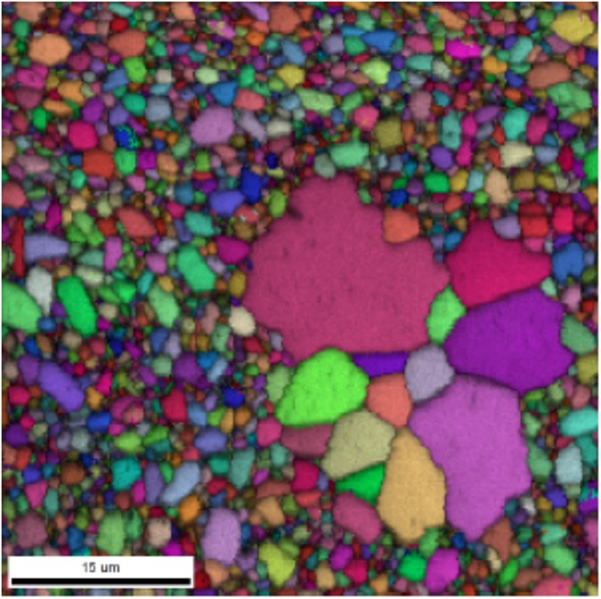
AGG occurs in a polycrystal when a small group of grains, typically having anisotropic boundary energies or mobilities, becomes relatively large by growing into the surrounding matrix of ‘‘normal” grains.24, 25 It is a ubiquitous phenomenon in many systems, especially thin films, and occurs, in some cases, due to the presence of impurity excesses (e.g., Ca or Si in alumina).26 AGG is found in both metallic and ceramic material microstructures and may have a significant impact on their electromechanical properties. Figure 1 shows a prototypical microstructure, as obtained from electron backscatter diffraction (EBSD), highlighting abnormal grains in a background of ‘‘normal grains” for an alumina sample.
A prototypical microstructure, as obtained from electron backscatter diffraction (EBSD), highlighting abnormal grains in a background of ‘‘normal grains” for an alumina sample. Reprinted with permission from Elsevier, Ltd27
In a recent paper, Lawrence et al.27 introduced a series of metrics that are useful in quantifying various microstructural aspects of AGG, and then employed a CCA to highlight the influence of processing variables on these metrics in doped aluminas.27 These metrics highlight specific features of the joint probability density function (pdf) p(G, a) of grain size, G, and aspect ratio, a, for a given microstructure, and, therefore, necessarily focus on grains in the tail of the distribution. More specifically, the metrics reflect the extreme events (i.e., large grains) that determine the shape of the tail in terms of conditional expectation values, and will be denoted here by {ϕ 1, ϕ 2, …, ϕ 5}. The object of the study by Lawrence et al. was to understand how the processing parameters for the doped aluminas, including compositions c (for such dopants as MgO, CaO, Na2O, and SiO2), temperature T and time t influence the aforementioned metrics. It should be noted that impurities often segregate to grain boundaries or other defects and may thereby affect thermomechanical and kinetic properties.28,29,30
In this study, we wish to identify which (possibly non-linear) combination(s) of processing variables is (are) most correlated with microstructural abnormality. To accomplish this aim, after the spark-plasma sintering of specialty alumina powders, we compiled statistics for microstructures associated with grain growth at some annealing temperature. The original work by Lawrence et al. was based on 33 samples; in this study we have augmented the original data set to obtain 68 independent samples. Each of the 68 independent specialty powders had a unique combination of processing variables, and the final microstructures had grain populations in the range of approximately 1000–9000 grains. For this analysis, it is convenient to define a set of input (i.e., processing) variables, \(\vec x\), and a set of output (i.e., metric) variables, \(\vec y\), as
where the composition subscripts denote dopant type.
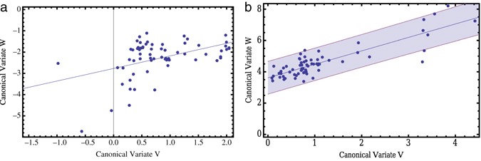
A CCA was performed using the data set described above. From this analysis, one finds a single pair of canonical variates having a (maximum) correlation coefficient of 0.59 and a p-value of 0.10 for the hypothesis test using Rao’s F-test.14 In Fig. 2a the corresponding canonical variates, V and W, are plotted for each of the data points, along with the associated regression line.
a The canonical variates V and W identified by a canonical correlation analysis of the 68 data points from Application 1. The regression line is also shown. b The same as for part a, except that these results are obtained after Monte Carlo simulation. Also shown are the corresponding regression line and a 95% confidence interval for the data (shaded region). The correlation coefficient is 0.86
To find variates having a stronger correlation, one can either use physical intuition to identify a new combination of variables or employ, for example, the CCAMC method. Based on the earlier work of Lawrence et al., one such variable that reflects perceived correlations, and identified via physical intuition, is the ratio \(r = {c_{{\rm{MgO}}}}{\rm{/}}\left( {{c_{{\rm{CaO}}}} + {c_{{\rm{Si}}{{\rm{O}}_2}}}} \right)\). With this guidance and after augmenting the input variable set with r, a CCA analysis yields a pair of canonical variates having a (maximum) correlation coefficient of 0.69 with a p-value of 0.02. To determine whether the CCAMC procedure can yield further improvement, consider the Padé functional form given in Eq. 5 with the variable set \(\left\{ {{c_{{\rm{MgO}}}},{c_{{\rm{CaO}}}},{c_{{\rm{Si}}{{\rm{O}}_{\rm{2}}}}}} \right\}\) and expansion exponent m = 1. These approximants replace r. These input variables were identified from the CCA as making significant contributions to the input canonical variate. Moreover, the inverse relationship between some pairs of variables suggests the Padé functional form. After approximately 100 simulations, each comprising 15,000 iterations, expansion coefficients were found yielding a maximum observed correlation coefficient of 0.86 with an associated p-value of 4 × 10⁻⁸. In Fig. 2b, the corresponding canonical variates are plotted for each of the data points, along with the associated regression line and a 95% confidence interval for the data. Thus, with relatively little computational effort, one can obtain well-correlated canonical variables using a trial function with the CCAMC methodology. These new variables facilitate experimental planning, as described below.
Application 2: Electrical and optoelectronic properties of thin films
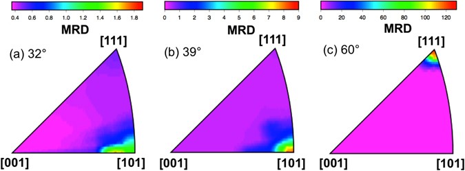
Thin-film solar cells, such as those based on, for example polycrystalline CuInSe2 absorbers, are of considerable technological interest given their relatively high conversion efficiencies.31 Indeed, many workers have sought to describe the role of grain boundaries in determining device performance in these systems.32 In a recent paper, Abou-Ras et al. examined the grain-boundary character of these films in relation to their electrical and optoelectronic properties for a relatively large number of grain boundaries.33 More specifically, EBSD was employed to acquire microstructural data that, in conjunction with an electron-beam-induced current (EBIC) analysis and a cathodoluminescence (CL) image study, permitted the correlation of boundary type with local electrical and optoelectronic properties. Figure 3 shows the distribution of disorientation axes for grain boundaries in polycrystalline CuInSe2, in multiples of a random distribution (MRD), presented as stereographic projections.
The distribution of disorientation axes for grain boundaries in polycrystalline CuInSe2, in multiples of a random distribution (MRD), presented as stereographic projections. The disorientation angles are a 32°, b 39°, and c 60°. Reprinted with permission from Elsevier, Ltd33
Several parameters were used to quantify the GBCD as extracted from EBSD maps, including, for a given boundary: the grain-boundary disorientation angle ψ, the three Rodrigues vector \(\overrightarrow R \) components of the disorientation and scalar measures of closeness k to the 〈100〉, 〈110〉, and 〈111〉 crystallographic directions. Our aim here is, as above, to to identify which (possibly non-linear) combination(s) of GBCD variables is (are) most correlated with electrical and optoelectronic properties. For this purpose, it is sensible to define sets of input and output variables, respectively, as
where the subscripts on k denote crystallographic directions and where ebic and cl are the EBIC and CL signals, respectively.
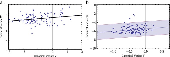
To identify those input and output variables that are most important in connecting microstructure to properties, one first performs a CCA using the variables given in Eq. 7. For concreteness, we consider a data set comprising 104 samples for non-twin boundaries. From this analysis, one finds a single pair of canonical variates that are maximally, though relatively weakly correlated, having a correlation coefficient of 0.26 and a large p-value of 0.88 for the hypothesis test using Rao’s F-test.14 (Given this p-value, one cannot reject the possibility that these variables are uncorrelated.) The canonical weights for the input and output variables are given in Table 1. In Fig. 4a, the corresponding canonical variates, V and W, are plotted for each of the data points, along with the associated regression line.
a The canonical variates V and W identified by a canonical correlation analysis of the 104 data points from Application 2. The regression line is also shown. b The same as for part a, except that these results are obtained after Monte Carlo simulation. Note the stronger dependence between the two variates as compared to those shown in a. Also shown are the corresponding regression line and a 95% confidence interval for the data (shaded region). The correlation coefficient is 0.56
From Table 1 it is evident that several of the input variables, given their relatively small canonical weights, make little contribution to the input canonical variate. This situation is, in fact, ideally suited to CCAMC as the trial function need only depend on a few input variables. We identify three input variables, namely the components of \(\vec R\), that have significant canonical weights and ask whether the addition of some (possibly) non-linear function of these variables would lead to a stronger correlation with the output variables. Consider, for example, the Padé functional form given in Eq. 5 with the variable set {R 1, R 2, R 3} and expansion exponent m = 1. After approximately 150 CCAMC simulations, each comprising 15,000 iterations, expansion coefficients were found yielding a maximum observed correlation coefficient of 0.56 with an associated p-value < 10−3. In Fig. 4b, the corresponding canonical variates are displayed for each of the data points, along with the regression line and a 95% confidence interval for the data. Clearly, this procedure has produced canonical variates with a substantially increased degree of correlation; moreover, the corresponding p-value gives one confidence that this correlation is real.
Discussion
We outlined above a MC-based methodology based on a CCA that permits one to identify non-linear functions of the variables that lead to strong input/output correlations. We then validated this CCAMC approach for two applications of technological relevance. The first application focused on the interdependence of processing and microstructural variables associated with doped polycrystalline aluminas, and the second related microstructural decriptors to the electrical and optoelectronic properties of thin-film solar cells based on CuInSe2 absorbers. In each case it was found that the CCAMC methodology was extremely useful in highlighting significant input/output correlations. It is expected that this methodology will also be useful in cases where the number of output variables exceeds the number of input variables given that underlying CCA analysis identifies correlated variates irrespective of which variables are labeled ‘‘input” or ‘‘output.’’
Having identified highly correlated variates, the information summarized in Figs 2 and 4 can be used for planning future experiments or for process control. For example, from Fig. 2 one can identify those processing variables (e.g., compositions) in Application 1 that, with a certain confidence, will produce a microstructure having target metrics (i.e., grain-size distributions). This capability greatly reduces the amount of experimentation required to produce microstructures having desirable characteristics.
One important issue that should be considered in applying the CCA or CCAMC technique is the adequacy of sample sizes. While there is no simple procedure for estimating sample size sufficiency, some authors have attempted to quantify the increase in sample size required as the number of variables increases.21, 34 In general, the minimum data requirements needed for these techniques depend on the reliability of the data. While relatively large sample sizes are, of course, desirable, and may be necessary in some cases, if there are strong correlations then relatively small samples sizes should detect them. As a practical matter, for Application 1 (AGG), it is very time consuming to perform the required microstructural analysis to obtain sensible grain probability distributions. Hence, we have taken the practical approach of recalculating the maximum eigenvalue and corresponding eigenvectors from CCA as we augmented our data set, starting with 33 samples and ending with 68 samples. The analysis is robust in that the same metrics are identified as contributing significantly to the canonical variates. Thus, we are confident that we are identifying the important factors that dictate AGG.
The CCAMC methodology has, of course, much broader application. Moreover, as noted above, it is readily parallelized, and, therefore, one can explore the parameter space associated with many different functional forms for the input variables. More rapid convergence to local extrema can also be achieved by employing extensions of the usual MC algorithm including, for example, force-biased MC.35 In this approach transition probabilities are modified by a knowledge of the instantaneous ‘‘force” associated with a configuration that, in this case, corresponds to the numerical derivative of λmax with respect to changes in the input variables. We are currently exploring other applications of the CCAMC methodology, as well as the role of CCAMC in guiding experimental processing in other contexts.
Data availability
The authors will make available, upon request, the data used in both applications described in this work. It is understood that the data provided will not be for commercial use.
References
Samudrala, S., Rajan, K. & Ganapathysubramanian, B. in Informatics for Materials Science and Engineering (ed. Rajan, K.) (Elsevier, 2013).
Lee, J. A. & Verleysen, M. Nonlinear Dimensionality Reduction (Springer, 2007).
Jackson, J. E. A User’s Guide to Principal Components (John Wiley and Sons, 2003).
Wu, K., Natarajan, B., Morkowchuk, L., Krein, M. & Breneman, C. M. in Informatics for Materials Science and Engineering (ed. Rajan, K.) (Elsevier, 2013).
Huang, W. & Yin, H. in Intelligent Data Engineering and Automated Learning-IDEAL 2009 (eds Corchado, E. & Yin, H.) (Springer-Verlag, 2009).
Meredith, W. & Millsap, R. E. On component analysis. Psychometrika 50, 495–507 (1985).
Gnanadesikan, R. & Wilk, M. B. in Multivariate Analysis II (ed. Krishnaiah, P. R.) (Academic Press, 1969).
Knapp, T. R. Canonical correlation analyis: a general parametric significance-testing system. Psych. Bull 85, 410–416 (1978).
Burges, C. J. C. Dimension reduction: a guided tour. Found. Trends Mach. Learn. 2, 275–365 (2009).
Akaho, S. in International Meeting of Psychometric Society (Osaka, Japan, 2001).
Balakrishnan, S., Puniyani, K. & Lafferty, J. Sparse additive functional and kernel CCA, in Proc. 29th International Conference on Machine Learning (Edinburgh, 2012).
Ivakhnenko, A. G. & Ivakhnenko, G. A. The review of problems solvable by algorithms of the group method of data handling (GMDH). Pattern Recogn. Image Anal 5, 527–535 (1995).
Schmidhuber, J. Deep learning in neural networks: an overview. Neural Networks 61, 85–117 (2015).
Jobson, J. D. Applied Multivariate Data Analysis, Vol. II (Springer-Verlag, 1992).
Gittins, R. Canonical Analysis: A Review With Applications In Ecology (Springer-Verlag, 1985).
Hartmann, A. K. & Weigt, M. Phase Transitions in Combinatorial Optimization Problems: Basics, Algorithms and Statistical Mechanics (Wiley-VCH, 2005).
Dehuri, S., Coello, C., Cho, S. -B. & Ghosh, A. in Swarm Intelligence for Multi-Objective Problems in Data Mining (eds Coello, C., Dehuri, S. and Ghosh, S.) 115–155 (Springer-Verlag, 2009).
Baker, G. A. & Graves-Morris, P. Padé Approximants 2nd edn, (Cambridge University Press, 1996).
Turut, V. & Bayram, M. Rational approximations for solving Cauchy problems. New Trend. Math. Sci. 4, 254–262 (2016).
Cuyt, A. A review of multivariate Padé approximation theory. J. Comp. Appl. Math 12,13, 221–232 (1985).
Thorndike, R. M. Correlational Procedures for Research (Gardner Press, 1978).
Press, W. H., Teukolsky, S. A., Vetterling, W. T. & Flannery, B. P. Numerical Recipes in Fortran: The Art of Scientific Computing 2nd edn, (Cambridge University Press, 1992).
Gentle, J. E. Matrix Algebra: Theory, Computations and Applications in Statistics (Springer, 2007).
Rollett, A. D., Srolovitz, D. J. & Anderson, M. P. Simulation and theory of abnormal grain growth-anisotropic grain boundary energies and mobilities. Acta Metall 37, 1127–1240 (1989).
Mullins, W. W. & Viñals, J. Linear bubble model of abnormal grain growth. Acta Mater. 50, 2945–2954 (2002).
Handwerker, C. A., Morris, P. A. & Coble, R. L. Effects of chemical inhomogeneities on grain growth and microstructure in Al2O3. J. Am. Ceram. Soc. 72, 130–136 (1989).
Lawrence, A., Rickman, J. M., Harmer, M. P. & Rollett, A. D. Parsing abnormal grain growth. Acta Mater. 103, 681–687 (2016).
Cho, J., Wang, C. M., Chan, H. M., Rickman, J. M. & Harmer, M. P. Improved tensile creep properties of yttrium- and lanthanum-doped alumina: a solid solution effect. J. Mater. Res. 16, 425–429 (2001).
Wang, C.-M., Cho, J., Chan, H. M., Harmer, M. P. & Rickman, J. M. Influence of dopant concentration on creep properties of Nd2O3-doped alumina. J. Amer. Ceram. Soc 84, 1010–1016 (2001).
Rickman, J. M., LeSar, R. & Srolovitz, D. J. Solute effects on dislocation glide in metals. Acta Mater. 51, 1199 (2003).
Jackson, P. et al. Effects of heavy alkali elements in Cu(In,Ga)Se2 solar cells with efficiencies up to 22.6%. Phys. Stat. Sol. (RRL), doi:10.1002/pssr.201600199.
Rao, U., Taretto, K. & Siebentritt, S. Grain boundaries in Cu(In,Ga)(Se,S)2 thin-film solar cells. Appl. Phys. A 96, 221 (2009).
Abou-Ras, D. et al. Grain-boundary character distribution and correlations with electrical and optoelectronic properties of CuInSe2 thin films. Acta Metall 118, 244–252 (2016).
Barcikowski, R. S. & Stevens, J. P. A Monte Carlo study of the stability of canonical correlations, canonical weights and canonical variate-variable correlations. Multivariate Behav. Res. 10, 353–364 (1975).
Rao, M. & Berne, B. J. On the force-bias Monte Carlo simulation of simple liquids. J. Chem. Phys. 71, 129–132 (1979).
Acknowledgements
We wish to thank Almatis, Inc. for kindly supplying the alumina samples for our microstructural analysis and for their guidance during this project. We also wish to thank D. Abou-Ras and colleagues for their data. We also acknowledge support from the Office of Naval Research under grant N00014-11-1-0678.
Author information
Authors and Affiliations
Contributions
J.M.R. is the primary author (and guarantor) of this work. He developed the formalism and did most of the analysis. Y.W. also performed some of the analysis, especially the CCA of the Application 1 data. A.D.R., M.P.H., and C.C. provided data and helped in the physical interpretation of the results presented here.
Corresponding author
Ethics declarations
Competing interests
The authors declare that they have no competing financial interests.
Additional information
Publisher’s note
Springer Nature remains neutral with regard to jurisdictional claims in published maps and institutional affiliations.
Rights and permissions
Open Access This article is licensed under a Creative Commons Attribution 4.0 International License, which permits use, sharing, adaptation, distribution and reproduction in any medium or format, as long as you give appropriate credit to the original author(s) and the source, provide a link to the Creative Commons license, and indicate if changes were made. The images or other third party material in this article are included in the article’s Creative Commons license, unless indicated otherwise in a credit line to the material. If material is not included in the article’s Creative Commons license and your intended use is not permitted by statutory regulation or exceeds the permitted use, you will need to obtain permission directly from the copyright holder. To view a copy of this license, visit http://creativecommons.org/licenses/by/4.0/.
About this article
Cite this article
Rickman, J.M., Wang, Y., Rollett, A.D. et al. Data analytics using canonical correlation analysis and Monte Carlo simulation. npj Comput Mater 3, 26 (2017). https://doi.org/10.1038/s41524-017-0028-9
Received:
Revised:
Accepted:
Published:
DOI: https://doi.org/10.1038/s41524-017-0028-9
This article is cited by
-
Autoantibodies targeting GPCRs and RAS-related molecules associate with COVID-19 severity
Nature Communications (2022)
-
The network interplay of interferon and Toll-like receptor signaling pathways in the anti-Candida immune response
Scientific Reports (2021)
-
In Situ Al-TiC Composites Fabricated by Self-propagating High-Temperature Reaction: Insights on Reaction Pathways and Their Microstructural Signatures
Metallurgical and Materials Transactions A (2020)
-
Materials informatics for the screening of multi-principal elements and high-entropy alloys
Nature Communications (2019)
-
Austenite Reconstruction Elucidates Prior Grain Size Dependence of Toughness in a Low Alloy Steel
Metallurgical and Materials Transactions A (2018)

