
Abstract
3D live imaging is important for a better understanding of biological processes, but it is challenging with current techniques such as spinning-disk confocal microscopy. Bessel beam plane illumination microscopy allows high-speed 3D live fluorescence imaging of living cellular and multicellular specimens with nearly isotropic spatial resolution, low photobleaching and low photodamage. Unlike conventional fluorescence imaging techniques that usually have a unique operation mode, Bessel plane illumination has several modes that offer different performance with different imaging metrics. To achieve optimal results from this technique, the appropriate operation mode needs to be selected and the experimental setting must be optimized for the specific application and associated sample properties. Here we explain the fundamental working principles of this technique, discuss the pros and cons of each operational mode and show through examples how to optimize experimental parameters. We also describe the procedures needed to construct, align and operate a Bessel beam plane illumination microscope by using our previously reported system as an example, and we list the necessary equipment to build such a microscope. Assuming all components are readily available, it would take a person skilled in optical instrumentation ∼1 month to assemble and operate a microscope according to this protocol.
Introduction
Fluorescence microscopy is an essential technique used in biological research to study the function and behavior of proteins and organelles of interest. The applications of live fluorescence imaging have expanded rapidly with the development of genetically encoded fluorescent probes and high-speed high-photon-efficiency cameras based on either CCD or scientific complementary metal-oxide semiconductor (sCMOS) technology, which have provided subcellular spatial resolution and single molecule sensitivity both in vitro and in vivo. However, in practice, live fluorescence imaging is usually limited to two spatial dimensions over a limited number of time points. Although 2D live imaging is capable of providing basic dynamic information of a living process, it is often incomplete and sometimes even misleading, for it only provides a partial representation of biological processes that evolve in 3D volumes. Therefore, high-resolution 3D live imaging is required to obtain a complete and accurate understanding of the biological processes being studied.
Challenges
3D live fluorescence imaging with subcellular spatial resolution is challenging because it requires a good balance between spatial resolution, optical sectioning, imaging speed, photobleaching, photodamage and other factors. First, nearly isotropic 3D spatial resolution, typically a few hundred nanometers, is necessary to recognize subcellular structures in 3D environments. Second, good optical sectioning capability is important for collecting images with high signal-to-noise ratio (SNR) and low out-of-focus background on thick samples or samples with densely labeled structures. Third, the imaging speed has to be high enough to capture the cellular and subcellular dynamics of interest, and the speed must increase as the spatial resolution improves to avoid blurred images. Fourth, the photobleaching and photodamage induced by the imaging system must be low enough to allow the specimen to be sampled densely enough and long enough to reveal the biological process of interest while leaving the specimen undisturbed so that the true physiological process is revealed. It is worth mentioning that this problem represents a huge challenge for many 3D live imaging techniques because at least ten times and as many as 100 times or more 2D image planes must be collected per 3D time point over typical cellular dimensions. Finally, these issues do not exist independently; they are often in opposition. For instance, higher spatial resolution almost always results in lower imaging speed, increased photobleaching and higher photodamage, and vice versa.
Conventional 3D live imaging techniques
Wide-field, confocal and two-photon (TP) fluorescence microscopy techniques, based on an epi-illumination configuration in which the same objective lens is used for excitation and detection, have been essential for 3D live imaging. However, a major problem of epi-illumination is that the excitation light penetrates through the whole sample axially when only the sample at the focal plane is in focus. The out-of-focus excitation produces high fluorescence background, wastes the limited fluorescence photon budget and introduces unnecessary photodamage. In addition, epi-illumination leads to anisotropic spatial resolution wherein the axial resolution is typically several times coarser than the lateral resolution. This anisotropy often limits the observation of the specimen to the lateral direction only, even when the imaging results are collected in 3D, because observations from other directions are less informative.
Each epi-illumination method has additional, specific limitations. Wide-field microscopy is not suited for 3D imaging on specimens more than a few micrometers thick because it is not able to reject fluorescence background created by this out-of-focus excitation. Confocal microscopy gains its optical sectioning capability by rejecting out-of-focus fluorescence by using a single pinhole or a pinhole array, but the improvement is accompanied by slower imaging speed, faster photobleaching and higher photodamage, thereby limiting the number of time points for live imaging. TP fluorescence microscopy achieves optical sectioning and simultaneously avoids an out-of-focus background through nonlinear absorption of the excitation, but the imaging speed is still limited by point-scanned detection using the photomultiplier tube (PMT), and nonlinear mechanisms introduce additional photodamage. It also has a limited multicolor imaging capability. In practice, confocal and, more recently, spinning-disk confocal microscopy have been the most common methods for live 3D imaging of cellular-scale specimens.
Selective plane illumination microscopy (SPIM)
Although the technique is a century old1, the rapid development of SPIM over the last decade2,3,4,5,6,7,8,9 was driven by the need for high-speed, low-photobleaching and noninvasive 3D live imaging. SPIM minimizes the out-of-focus excitation by using two objectives with optical axes orthogonal to each other separately for excitation and detection. The sample is illuminated from the side by sending a sheet of excitation light into the sample, so that the illumination is confined near the focal plane of the orthogonal detection objective (Fig. 1a). In comparison with epi-illumination methods, SPIM has the following advantages. First, the confined excitation provides optical sectioning automatically by producing minimal out-of-focus fluorescence background. Second, the method is as fast as conventional wide-field detection, as fluorescence is imaged across the entire excitation plane simultaneously. Third, if the sheet thickness is comparable to or thinner than the depth of focus, the overall axial resolution is improved. Finally, SPIM has much lower photobleaching because only the fluorophores near the detection focal plane are illuminated, and this confinement of excitation to one plane also mitigates photodamage.

(a,b) The light sheet of conventional plane illumination can be created by a sheet-like nonscanning line focus (a) or by scanning a focused Gaussian beam to produce a virtual light sheet (b). (c) Comparison of Gaussian beams at 0.5 (top) and 0.15 (middle) excitation NA and a Bessel beam with 0.5 NAOD and 0.46 NAID (bottom). The Bessel beam has a central peak slightly narrower than even the high-NA Gaussian beam, but it is at the same time as long as the low-NA Gaussian beam. However, it also has strong side lobes, which must be taken into account when it is used for plane illumination.
In SPIM, the light sheet can be a real one, existing simultaneously across the illumination plane (such as that produced by a cylindrical lens)2,3, or a virtual one, created by serially scanning a long Gaussian beam produced at a low numerical aperture across the plane4,5,6,7,8,9. A real light sheet typically requires much lower peak intensities so that it produces less photodamage, whereas a virtual light sheet gives more control over the size and the intensity profile of the illuminated region.
Conventional SPIM has proven to be most successful for the 3D live imaging of multicellular specimens with single-cell resolution. The 3D spatial resolution of SPIM is determined by both the excitation and detection numerical apertures (NAexc and NAdet, respectively). The lateral resolution is the same as the conventional diffraction limit of the wide-field microscopy,  , where λem is the wavelength of the emitted fluorescence. The axial resolution of
  is related to boththe thickness of the illumination light sheet,
  , and the axial resolution of detection objective,
  , where λexc is the excitation wavelength, n is the refractive index of the imaging buffer, and θdet = sin−1(NAdet/n) is the half-angle of light collection in the imaging buffer. Clearly, the axial resolution becomes higher with higher NAexc, corresponding to a thinner light sheet. More importantly, the missing cone of the wide-field detection optical transfer function (OTF) is filled in SPIM by the excitation light sheet, which is the fundamental reason why SPIM has optical sectioning capability.
To obtain uniform axial resolution and optical sectioning capability, the light sheet thickness has to be uniform across the entire imaging field. However, there is a trade-off between the length of a Gaussian light sheet and its thickness owing to the diffraction of light: a light sheet of minimum thickness of 2wo varies in thickness by a factor of  over a distance defined by the Rayleigh length,
  . For instance, a light sheet ∼2 μm thick is required to cover a ∼30-μm field of view with a 488-nm excitation wavelength. Therefore, Gaussian light sheets of 2–10 μm in thickness are commonly used. The axial resolution with such light sheets remains dominated by the axial resolution of the detection objective alone, and hence conventional SPIM (without sample rotation)4,5,6,7,8,9 rarely reveals as much subcellular detail in the axial direction as a confocal microscope at a high NA. To improve the axial resolution to the point at which the 3D spatial resolution is nearly isotropic, and to maximize the advantages of optical sectioning, thinner illumination light sheets are required.
Bessel beam plane illumination microscopy
We introduced Bessel beams10 to overcome the trade-off between the length and thickness of conventional Gaussian 2D beams and 1D light sheets. Below we discuss the three operational modes of Bessel beam plane illumination microscopy (Table 1): Bessel beam plane illumination (sheet-scan mode), TP Bessel beam plane illumination (TP excitation sheet-scan mode), and Bessel beam structured plane illumination (Bessel structured illumination microscopy mode).
Bessel beam plane illumination. An ideal Bessel beam, one of the class of so-called 'nondiffracting beams', propagates indefinitely with no change in its cross-sectional intensity profile, I(r)∝|Jo(αr)|2, where Jo(αr) is the zero-order Bessel function of the first kind11. Thus, the central peak of this ideal beam is surrounded by an infinite series of concentric side lobes of decreasing peak intensity, but with equal integrated intensity in each lobe. The ideal beam would exist at the front focal plane of a lens illuminated at its back focal plane with an infinitesimally thin annulus of light.
In practice, this is not possible. An experimental 'Bessel beam' is actually a Bessel-Gauss beam created with annular illumination of finite width. For a given NAexc, the thinner the annulus, the more Bessel-like the beam becomes, the longer its axial extent (i.e., the beam length), and the more energy exists in the side lobes (Fig. 1b). Conversely, the wider the annulus, the more Gaussian the character of the beam, the shorter its axial extent, and the smaller the side lobe energy. In either limit, the width of the central peak, and hence the thickness of the central core of a virtual light sheet made by sweeping the beam, is proportional to  . However, for longer beams that cover larger fields of view, the increased side lobe energy results in increased energy in excitation tails on either side of this central core. Hence, a key aspect of Bessel beam plane illumination is to use a beam that is only as long as is necessary to cover the desired field of view and no longer. Beyond this, other tricks, such as nonlinear excitation or structured illumination, are needed to mitigate the effects of the reduced optical sectioning and increased out-of-focus background and photobleaching resulting from the residual side lobe energy.
TP Bessel beam plane illumination. Although substantial integrated energy can exist in the side lobes, the intensity I of the central peak of even an ideal Bessel beam is much greater than that of any of the side lobes. By using a nonlinear process S∝In with n ≥ 2, the signal S generated at the central peak dominates and the contribution from the side lobes is minimal. For example, with TP excited fluorescence the signal can be constrained to a thin beam of several hundred nanometers thick but tens of micrometers long. Scanning this beam produces a virtual light sheet having negligible out-of-focus fluorescence background. At NAdet = 1.1, this TP mode offers a nearly isotropic 3D spatial resolution of ∼230 nm laterally and ∼350 nm axially, as well as excellent optical sectioning capability and fast imaging speed up to hundreds of planes per second10. Its limitations are a relatively high requirement on the brightness of fluorophores (compared with linear excitation), a limited capability for live imaging with multiple colors simultaneously and the possibility of additional nonlinear photodamage mechanisms. In contrast, as with conventional TP imaging, the IR excitation light that is typically used can penetrate further into multicellular organisms and tissues than visible excitation. As a result, the TP mode is a good option when imaging deeply into scattering and/or aberrating specimens, and it can produce substantially thinner virtual light sheets than Gaussian TP beams12 over a comparable field of view.
Bessel beam structured plane illumination. The combination of Bessel beam plane illumination with structured illumination microscopy (SIM) provides another avenue to minimize the negative effects of the Bessel beam side lobes. In conventional wide-field SIM, a periodic excitation pattern of period T is applied to the sample, and a series of raw images are acquired as the pattern is moved relative to the sample in N equal steps of T/N. One of two different algorithms is then used to reconstruct an image of the sample at the focal plane.
In optical sectioning SIM (OS-SIM)13, the N raw images In are combined to create the reconstructed image  . The effect of this algorithm is to subtract the contributions from the out-of-focus signal in the N raw images, which is much more weakly modulated by the applied excitation pattern than the in-focus signal.
In super-resolution SIM (SR-SIM)14, N raw images are again collected, which generates a series of N equations that can be combined with the N unknowns (given by the frequency-shifted copies of the sample structure encoded by the patterned excitation) to produce a reconstructed image Ifinal beyond the diffraction limit of the detection objective in the patterned direction and, in 3D SIM15,16, along the detection axis as well.
To apply either SIM approach to Bessel beam plane illumination, the beam is moved in discrete steps, rather than continuously, across the excitation plane to create a virtual grating pattern for SIM (Fig. 2). In contrast to wide-field OS-SIM, in which usually only N = 3 images are acquired per plane (to minimize the time per plane needed to achieve optical sectioning), Bessel OS-SIM requires the full complement of N = H + 2 raw images per plane for the reconstruction to be uniform across the entirety of Ifinal (i.e., for the point spread function (PSF) after reconstruction to be spatially invariant). Although this would suggest using a pattern of small period T containing only one harmonic H to minimize the number of raw images required, in thick or densely labeled samples the contrast of the applied pattern relative to the out-of-focus background due to the Bessel side lobes is often too low in this limit to provide a successful reconstruction with an acceptable SNR. Thus, in practice, the excitation period T is tailored to each sample individually until it is just large enough to provide sufficient contrast in the raw images and acceptable SNR in Ifinal. For most samples, periods corresponding to N = 7 or 9 images per plane are sufficient. The primary advantages of Bessel plane OS-SIM10 are its marked reduction in out-of-focus background in the reconstructed image, and its computational simplicity: it can be used to provide real-time feedback as the data are acquired concerning sample viability, brightness and optimal imaging conditions. One disadvantage of the technique is that the nonlinearity inherent in the absolute value function used in the OS-SIM reconstruction leads to image artifacts. Another is that the OS-SIM algorithm uses the signal encoded by only two of the N = 2H + 1 frequencies in the excitation OTF (Fig. 2b, right) in the reconstruction, or only a small fraction of the total signal. As a result, high excitation power and longer periods requiring more images per plane are often needed to achieve acceptable SNR, leading to low imaging speed, fast photobleaching and high photodamage in the context of live imaging.

(a) The structured illumination pattern is the convolution of the excitation beam intensity profile and a periodical modulation function, M(x), in real space. (b) The Fourier transform of the illumination pattern is the product of the Fourier transform of the excitation beam intensity profile and the Fourier transform of the modulation function,  , in frequency space. The number of harmonics contained in the illumination pattern is determined by the excitation beam NAOD and the modulation period T. For the sheet-scan mode, T needs to be less than λ/(2NAOD). (c) The normalized intensity profile of each modulation harmonic with excitation wavelength 488 nm, NAOD = 0.5 and T = 1.8 μm. The DC harmonic contains highest axial spatial frequency information, but provides the worst optical sectioning capability. All AC harmonics provide better optical sectioning capability but lower axial frequency limits compared with the DC harmonic. (d) The corresponding OTF of each modulation harmonic, which is the convolution of the wide-field detection OTF with each modulation harmonic in frequency space. A gamma value of 0.5 is applied to the DC harmonic OTF to make the high-frequency contents visible. The Bessel SR-SIM OTF is the sum of all OTFs at the corresponding position of each OTF in frequency space. The fundamental harmonic OTF gives the best optical sectioning, and the highest frequency harmonic gives the maximal resolution extension in the x direction.
Bessel plane SR-SIM17 works much better for image reconstruction. The N raw images per plane are acquired identically to Bessel plane OS-SIM, whereas the reconstruction uses the same algorithm as 3D wide-field SR-SIM. Unlike OS-SIM, this algorithm uses the signal encoded by all N = 2H + 1 frequencies of the excitation OTF and places the frequency-shifted sample information contained in each in its appropriate place in an expanded frequency space representation of the sample. This has three beneficial consequences. First, much lower excitation power and fewer raw images per plane are required to achieve an acceptable SNR. This leads to faster imaging, less photobleaching and reduced phototoxicity. Second, the reconstructed image faithfully represents the true sample structure at all length scales down to the resolution limit of the method. Third, when applied to 3D image stacks, this resolution limit is itself extended beyond the classical diffraction limit in both the patterning direction (defined as the x direction) and in the axial direction orthogonal to the excitation plane (the z direction).
Quantitatively, the resolution limit of Bessel plane SR-SIM in the x direction is given by  , and in the z direction by
  . The resolution along the beam propagation direction (the y axis) remains diffraction limited:
  .
.
In our instrument, we chose NAdet = 1.1 to maximize the signal collection efficiency within the constraints of using a water-dipping (i.e., no cover glass) objective with a long working distance of 2 mm to accommodate large specimens. Owing to the additional constraints that the excitation and detection objectives must be orthogonal, and that the excitation and detection illumination cones cannot intersect, the maximum excitation NA is limited to NAexc = 0.65. We had a custom achromatic long-working-distance water-dipping objective fabricated to reach this limit in order to achieve the highest possible 3D resolution. Specifically, with these objectives we can reach  nm (equivalent to a wide-field microscope of NAdet = 1.75),
  nm, and
  nm by Bessel plane SR-SIM when imaging green (e.g., GFP) fluorescence.
Implementing multiple scanning beams to reduce photobleaching and phototoxicity
In fluorescence imaging, photobleaching and phototoxicity depend not only on the total integrated dose of excitation photons delivered to the sample but also on the instantaneous peak intensity, as nonlinear damage mechanisms can have an important role. This poses a considerable problem for plane illumination microscopy with a virtual scanned light sheet, as the excitation energy is then concentrated in a line that must sweep rapidly across the illumination plane in the limited time allotted for collecting each 2D image of a 3D stack. Indeed, as the light sheet becomes thinner and the imaging speed becomes higher (twin goals of Bessel beam plane illumination), the problem rapidly becomes more acute. For example, a Bessel beam of central peak width of 0.5 μm scanning at 50 planes/s across a 50-μm field of view will illuminate any given voxel for only 200 μs; therefore, the beam intensity must be high enough to produce enough fluorescence photons within this time to reach an acceptable SNR.
To mitigate this problem, we have used parallel arrays of J Bessel beams. Each beam then needs to scan over only 1/J of the original field of view in the same time, requiring only 1/J as much power in each beam to produce the same amount of signal per unit time across the whole plane. Although the total dose delivered to the sample is then the same as with a single beam, the reduction in peak intensity often has a profound effect on prolonging cell viability. An ancillary advantage of Bessel plane SIM is that each beam need be moved in only 1/J as many discrete steps. As the response time of the galvanometer mirror used for this purpose can be a rate-limiting factor, this also opens the door to faster Bessel SIM imaging.
We create these linear beam arrays using a commercial Dammann grating-based diffractive optical element (DOE) that splits an incoming beam into a fan of J outgoing beams of equal intensity at equal angular spacing. When placed next to an annular mask conjugate to the rear pupil of the excitation objective, this creates an array of J parallel Bessel-Gauss beams across a plane within the sample. However, it is important that these beams be separated sufficiently so that their side lobes do not overlap appreciably, because the DOE-generated beams do not have a well-defined phase relationship with one another, and they therefore produce nonperiodic speckle patterns when they mutually interfere.
Summary of modes and applications of Bessel beam plane illumination microscopy
Table 1 summarizes the various operational modes of Bessel beam plane illumination microscopy. The linear swept sheet mode (Bessel beam plane illumination) offers high speed and multicolor capability, but its optical sectioning capability is compromised by the Bessel beam side lobes. This makes it difficult to extract information even close to the approximately 3× axial resolution gain that it theoretically provides over conventional wide-field microscopy. Nevertheless, it can still address important biological questions18,19 when the side lobe background is not a concern. The TP mode (TP Bessel beam plane illumination) offers high-speed and near-isotropic 3D resolution, but with limited multicolor capability20. It is the mode of choice for deep imaging, owing to the better penetration of its IR excitation in scattering and/or aberrating tissues. The Bessel plane OS-SIM mode provides good optical sectioning, but it is very photon inefficient and prone to artifacts. It is used primarily for real-time assessment of Bessel SIM images for later off-line processing by the SR-SIM algorithm. This Bessel plane SR-SIM mode (Bessel beam structured illumination) provides the best resolution: slightly beyond the diffraction limit in the x direction and nearly 3× beyond the wide-field limit in z. It also offers good photon efficiency, accurate 3D sample reconstruction and multicolor capability. Its primary disadvantages are the added time required to take N images per plane instead of one, and the noise introduced if the higher spatial frequencies are reconstructed at greater amplitudes than those that the SNR should allow. Finally, although it is not discussed here, the TP mode and Bessel plane SR-SIM mode can be combined to merge the high resolution of Bessel plane SR-SIM with the good depth penetration of two-photon excitation17. Together, these modes provide a range of solutions that balance 3D spatial resolution, optical sectioning, imaging speed, photobleaching and photodamage for different live fluorescence imaging applications. In comparison with conventional 3D fluorescence imaging techniques, especially confocal fluorescence microscopy, Bessel beam plane illumination offers better performance by all these metrics.
Limitations of Bessel beam plane illumination microscopy
Bessel beam plane illumination microscopy has several limitations. First, although Bessel plane SR-SIM can extend resolution in the x and z directions slightly beyond the diffraction limit, Bessel beam plane illumination is not capable of extending into the sub-100 nm regime without being combined with other super-resolution methods21,22,23,24 such as photoactivated localization microscopy (PALM), stimulated emission depletion (STED) microscopy or nonlinear SIM. Second, the imaging depth is usually limited to ∼50 μm or less below the sample surface owing to optical aberrations and light scattering induced by the sample. The so-called 'self-healing' properties of Bessel beams do not improve the imaging depth because the conical shell of light that forms the Bessel beam is also aberrated or scattered within such samples25. Thicker Bessel-Gauss beams (i.e., lower NAexc) with less side lobe excitation (i.e., thicker annulus width) are often preferred in these circumstances, although the axial resolution is poorer. Third, the sample mounting conditions are different from those to which most biologists are accustomed. Samples are mounted on 5- or 8-mm-diameter cover glasses in order to fit in the space between the two objectives. In addition, because these are water-dipping lenses, the specimen cannot be sandwiched between cover slips: nothing can interfere in the half-space above the cover slip. Fourth, the cover slip must be placed directly into the imaging chamber clipped in a custom holder instead of into a conventional Petri dish. In its current incarnation, the chamber contains 10–35 ml of imaging buffer, which is advantageous for maintaining temperature, pH and dissolved CO2 levels, but it can be disadvantageous when one wishes to add expensive drugs in perturbation experiments. Finally, every few weeks this chamber must be disassembled and thoroughly cleaned to prevent contamination, a process that requires several hours of skilled realignment of the objectives and associated optics.
Spatial resolution and optical sectioning capability of Bessel beam plane illumination microscopy
Axial resolution and optical sectioning. Two concepts, axial resolution and optical sectioning capability, are particularly important in 3D fluorescence imaging, and yet they are often confused with each other. The axial resolution defines the smallest axial separation at which two features can be resolved under conditions of negligible noise, whereas the optical sectioning capability is a measure of the ability of a microscope to reject out-of-focus fluorescence background. They are, however, related, as increasing fluorescence background from poorer optical sectioning will set a practical limit on the axial resolution that is coarser than the theoretical one.
These concepts can perhaps be better understood in frequency space. A microscope image is the convolution of the microscope PSF and the fluorescence emission pattern of the object under investigation, D(r) = H(r)⊗E(r), where D(r) is the recorded image, H(r) is the PSF of the microscope and E(r) is the emission pattern. By the convolution theorem, this is equivalent to:  , where
  ,
,  , and
, and  are the Fourier transforms of D(r), H(r) and E(r), respectively.
  defines the microscope's OTF. It is nonzero only for a contiguous region of k space centered at k = 0 and, within this region, it generally decreases with increasing distance from the origin. Thus, the microscope acts as a low-pass filter, and the recorded image that we see is a blurred copy of emission pattern of the sample that we wish to know. Broad features corresponding to low k are more strongly represented in the image than fine features corresponding to high k, and no features corresponding to k values outside the nonzero portion of the OTF will appear at all. In other words, the nonzero region of the OTF defines the pass-band of the microscope and the boundaries of this region, called the support of the OTF, define the best possible spatial resolution theoretically obtainable in any given direction.
Seen in this light, the optical sectioning capability of a microscope is a reflection of how quickly its OTF rolls off to zero in the axial direction: even with the same ultimate limit of support and hence the same theoretical axial resolution, an OTF that maintains significant amplitude at high kz will outperform one with lower amplitudes at the same kz, as the information in the image will then be weighted more highly to the in-focus fluorescence emitted closer to the focal plane than to the out-of-focus fluorescence from further away. In particular, in live fluorescence imaging, the number of photons in the image is always limited by photobleaching and phototoxicity, so the attenuated high-frequency signal is often submerged in noise from the out-of-focus background, thereby making the theoretical resolution unachievable in practice. Thus, the optical sectioning capability of a microscope is at least as important as its theoretical axial resolution limit.
Axial resolution and optical sectioning capability of Bessel beam plane illumination. The axial resolution and optical sectioning capability of Bessel beam plane illumination is determined by the convolution of the traditional wide-field detection OTF with the excitation OTF defined by the Bessel beam and the microscope's mode of operation. The detection OTF has a 'missing cone' of axial information, which, by itself, leads to poor optical sectioning and a substantial out-of-focus background. However, the OTF of the excitation plane fills in this missing cone, reducing background and often improving the practical limit of axial resolution.
In real space, the Bessel plane excitation function I(r) is the convolution of the fluorescence emission function created by a single Bessel-Gauss excitation beam B(r) and a function M(x) that describes how the intensity of this beam is modulated as it sweeps in the x direction to create a virtual excitation plane, I(r) = B(r)⊗M(x), or, in Fourier space:  . For long Bessel-Gauss beams, we can assume that the illumination is uniform along the propagation direction y over cellular-sized fields: B(r) ≈ B(x, z). In this case, for each of the modes described above and summarized in Table 1, we have:
Linear swept sheet: 
Linear Bessel plane SIM:


Two-photon swept sheet: 
Two-photon Bessel plane SIM:


where, as above, T is the period of the SIM grating pattern, and H = floor [T/(0.5λexc/NAexc)] is the number of harmonics in this pattern when the pattern is created by moving the beam in discrete steps of length T. Note that in all of these expressions, , is of the form:

where j = 1 or 2 (linear or two photon, respectively) and m = 0 or m >0 (swept or SIM modes, respectively). In addition, the Bessel plane excitation function I(r) creates a fluorescence emission pattern E(r) in a sample with a fluorophore distribution S(r): E(r) = S(r)I(r). Thus, referring back to the beginning of this section:

However, as the excitation plane remains coincident with the detection focal plane throughout the capture of the 3D stack, it has been shown that this reduces to14:

In physical terms, this expression states that the recorded image is a sum of 2H + 1 copies of the sample structure, shifted in frequency space in successive increments of Δkx = 1/T, and each weighted by the strength Cm of the mth band of the periodic excitation as well as by an effective OTF,  , which serves as a filtering function of finite bandwidth.
Examples of Om(k) for different m and j = 1 (linear excitation) are shown in Figure 2d. The OTF corresponding to the DC harmonic is equivalent to the overall OTF of the swept sheet mode (i.e., where H = 0, so only the DC harmonic remains). It gives the highest theoretical axial resolution, but has very poor sectioning capability, as evidenced by the strong peak at k = 0. This is a reflection of the strong out-of-focus background from the side lobes of the swept Bessel beam. Moving outward from the DC band, successive OTFs Om(k) corresponding to bands at higher and higher |kx| provide less and less axial resolution but more and more resolution in the x direction. Together, in the above sum, they are capable of providing substantial extension of resolution in the xz plane beyond the wide-field diffraction limit of the detection objective alone (Fig. 2d, right). To do so, however, the SNR of the collected images and the coefficients Cm must be sufficiently large to detect their contributions over the much stronger DC band, which has the dominant peak at k = 0.
There are three ways to increase the strengths of the AC weighting terms CmOm(k) relative to the DC term. The first is to write a stepped pattern of longer period T, having more harmonics H. It is realized by parking the Bessel beam at discrete positions of fixed spacing T during scanning, while turning off the beam at all other points in between. This tends to spread the spectral energy out from the DC band across the additional harmonics. In addition, the added harmonics at lower spatial frequencies tend to have higher coefficients Cm than those closer to the diffraction limit. Of course, more harmonics require more images D(r) to reconstruct S(r); typically 5–7 raw images are required per plane, which slows the imaging speed proportionally relative to the sheet-scan mode. In addition, the information encoded by the weak higher harmonics (which provide the greatest resolution extension in the x direction) may not be recoverable. Thus, another approach is to sweep the beam continuously, but to modulate its amplitude with the acousto-optical tunable filter (AOTF) in a sine pattern of period T. This generates only H = 1 harmonic, with relatively large Cm for m = ±1, as the associated bands are at low |kx|. It requires only three images D(r) to reconstruct S(r), so that the imaging speed is only three times slower than that of the sheet-scan mode. It also induces less photodamage compared with the stepped mode, yet it extends the resolution in the z direction just as much, as both approaches exploit the high |kz| extent of the first harmonic. However, this sine modulation mode does not provide much resolution improvement in the x resolution as the first harmonic is restricted to low |kx|. The final approach is to reduce the spectral energy in the DC term, particularly in the peak near k = 0. This can be done by choosing a Bessel-Gauss beam having less side lobe excitation, and hence an out-of-focus background contributing to this peak. Of course, this means choosing a shorter beam and reducing the field of view in the y direction.
Materials
REAGENTS
-
Alexa Fluor 488, hydrazide, sodium salt (Invitrogen, cat. no. A10436), see Reagent Setup
-
Alexa Fluor 568, hydrazide, sodium salt (Invitrogen, cat. no. A10437), see Reagent Setup
-
Alexa Fluor 647 cadaverine, disodium salt (Invitrogen, cat. no. A30679), see Reagent Setup
-
FluoSpheres carboxylate-modified microspheres, 0.1 μm, yellow-green fluorescent (Invitrogen, cat. no. F8803) see Equipment Setup
-
FluoSpheres carboxylate-modified microspheres, 0.1 μm, red fluorescent (Invitrogen, cat. no. F8801) see Equipment Setup
-
FluoSpheres carboxylate-modified microspheres, 0.2 μm, dark red fluorescent (Invitrogen, cat. no. F8807) see Equipment Setup
-
Dulbecco's PBS, 1× PBS (Cellgro, cat. no. 21-031)
-
Poly-D-lysine hydrobromide (Sigma-Aldrich, cat. no. P0899)
-
Cell-Tak cell and tissue adhesive (BD Biosciences, cat. no. 354240)
-
Hydrogen peroxide, 50% (wt/vol) (H2O2)
Caution
It is corrosive.
-
Ammonium hydroxide, 30% (wt/vol) (NH4OH)
Caution
It is corrosive.
EQUIPMENT
Critical
The opto-mechanical model for our Bessel beam plane illumination microscope and the associated mechanical drawings for custom components are available from HHMI after execution of a nondisclosure agreement (NDA)
Critical
We have listed the equipment used to build our microscope. However, unless otherwise specified, most items can be replaced with products from other vendors that give comparable performance.
-
Optical table (TMC, optical tabletop, cat. no. 784-455-02R, optical table leg, cat. no. 14-417-35)
-
Optical breadboard (ThorLabs, cat. no. PBH11106)
Laser sources for linear excitation and TP excitation
-
405-nm laser (Coherent, CUBE, 405-100C)
-
488-nm laser (Coherent, Sapphire LP, 200 mW)
-
561-nm laser (Coherent, Sapphire LP, 200 mW)
-
640-nm laser (Coherent, CUBE 640-100C)
-
Ultrafast Ti-sapphire laser (Coherent, Chameleon Ultra II Ti-Sapphire laser)
Laser intensity modulation devices
-
AOTF, for 405 nm∼650 nm continuous-wave (CW) lasers (AA Opto-Electronic, cat. no. AOTFnC-400.650-TN)
-
Pockels cell (Conoptics, cat. no. M350-80LA-02, for the Ultrafast laser)
Laser, objective and sample-scanning devices
-
Scanning galvanometer mirrors, 3 mm square, protected silver (GM-Z, GM-X, Cambridge Technology, cat. no. 6215HP-1HB)
-
Objective scan piezo, 100-μm range (Physik Instrumente, cat. no. P-726.1CD PIFOC)
-
Objective scan piezo controller (Physik Instrumente, cat. no. E665)
-
Sample scan piezo, 100-μm range (Physik Instrumente, cat. no. P-621.1CD)
-
Sample scan piezo controller (Physik Instrumente, cat. no. E625)
Objectives
-
Excitation objective (EO, Nikon CFI Apo 40XW near-infrared (NIR), 0.8 NA, 3.5 mm working distance (WD) or Special Optics, custom objective, cat. no. HH-PO159319, water dipping, 0.65 NA, 3.74 mm WD)
-
Detection objective (DO, Nikon CFI Apo 40XW NIR, 0.8 NA, 3.5 mm WD or Nikon CFI Apo LWD 25XW, 1.1 NA, 2 mm WD)
-
Wide-field objective (WO, Olympus, UMPLFLN 20XW, 0.5 NA, 3.5 mm WD)
Detection camera
-
Electron multiplying (EM)-CCD camera (Andor Technology, iXon3 885, high quantum efficiency)
-
sCMOS camera (Hamamatsu, ORCA Flash 4.0, higher speed, larger filed of view)
-
Alignment inspection camera, wide-field camera (AVT Guppy F-146 Firewire, Edmund Optics, cat. no. 59-731)
Laser shaping devices
-
DOE (Holo/OR, cat. no. MS-107-Q-Y-A, to create seven Bessel beams simultaneously)
-
Custom aluminum-coated quartz annulus mask (AM, Photo Sciences, to create an annular laser beam)
-
Axicon, 0.5° (AX, Thorlabs, cat. no. AX2505-B, to create an annular focus)
System control devices
-
Computer, >48 GB RAM and >1 TB hard drive (Supermicro, cat. no. SYS-7046GT-TRFP. Recommended configuration: 2 Xeon 5680 CPU)
-
Rack-mount LCD monitor (Crystal-Image Technologies, cat. no. RMPW-161-19))
-
Signal generation board (National Instruments, cat. no. PCIe-7852R)
-
Scaling amplifier mainframe (Stanford Research Systems, cat. no. SIM900)
-
Scaling amplifier (Stanford Research Systems, cat. no. SIM983)
-
Control software written in Labview 2013 (available from HHMI upon execution of an NDA). National Instruments (NI) Labview, the NI Vision Development Mmodule and the NI field-programmable gate array (FPGA) module are required to run the software
Filters and dichroic
-
Neutral density filter wheel (Thorlabs, cat. no. NDM2)
-
Lasermux laser combining filter (LM, Semrock, cat. no. LM01-427-25)
-
Lasermux laser combining filter (LM, Semrock, cat. no. LM01-503-25)
-
Lasermux laser combining filter (LM, Semrock, cat. no. LM01-613-25)
-
Short-pass dichroic beam splitter (DC1, Semrock, cat. no. FF670-SDi01-25x36)
-
Multiband laser-flat dichroic beamsplitter (DC2, Semrock, cat. no. Di01-R405/488/543/635-25×36)
-
Band-pass filter (Semrock, cat. no. FF01-525/50-25), to be used as the emission filter in the detection path for fluorescent probes with emission wavelength at ∼525 nm. For instance, GFP, mEmerald and Alexa Fluor 488
-
Band-pass filter (Semrock, cat. no. FF01-600/37-25), to be used as the emission filter in the detection path for fluorescent probes with emission wavelength at ∼600 nm. For instance, RFP, tdTomato, mCherry and Alexa Fluor 568
-
Multiband band-pass filter (Semrock, cat. no. FF01-523/610-25), to be used as the emission filter for dual-color imaging by using fluorescence probes with emission wavelength at ∼525 nm and ∼600 nm
-
Multiband band-pass filter (Semrock, cat. no. FF01-440/521/607/700-25), to be used as the emission filter in the wide-field detection path
Other optical components
-
Achromatic lenses (focal lengths should be selected on the basis of the optical system design)
-
Optical mirrors (protected silver)
Sample and sample mounting
-
Sample. Samples should be prepared, fixed and labeled using the same methods used for regular fluorescence microscopy (wide-field, confocal)
-
Sample coverslip (Warner Instruments, cat. no. CS-5R/CS-8R)
-
Sample mounting. Cellular specimens should be cultured directly on either 5-mm- or 8-mm-diameter coverslips, which can then be clipped onto the top surface of the specimen holder and mounted in the chamber with the sample side facing the excitation and detection objectives. Multicellular organisms, such as Caenorhabiditis elegans or Drosophila embryos, can be attached to the cover slip with poly-D-lysine, tissue adhesive or double-sided tape. Larger samples can be mounted with agarose gel according to published protocols4
REAGENT SETUP
Alexa Fluor solutions
-
Prepare separate 0.5 μg/ml solutions of Alexa Fluor 488 hydrazide sodium salt in H2O for system alignment using the 488-nm CW laser and the Chameleon ultrafast laser at 920 nm. Prepare Alexa Fluor 568 hydrazide sodium salt solution and Alexa Fluor 647 cadaverine, disodium salt solution with the same concentrations for the alignment of the 568-nm CW laser and the 647-nm laser alignment, respectively.
EQUIPMENT SETUP
Preparation of cleaned cover slips
-
Prepare a 150 ml mixture solution of hydrogen peroxide (H2O2, 50%), ammonium hydroxide (NH4OH, 30%) and H2O in a ratio of 1:1:5 by volume. Soak the coverslips in the solution for 12 h. Rinse the coverslips with H2O and sterilize by flaming them with methanol. The cleaned coverslips can be stored in sterile containers for up to 1 week.
Caution
These are corrosive chemicals; coverslips should be prepared in a chemical hood.
Preparation of fluorescent bead sample for microscope alignment
-
Dilute fluorescent microsphere solution of the appropriate color for the laser wavelength of interest 106× in H2O. Add ∼30 μl of a solution of 0.1 mg/ml poly-D lysine in water on top of a cleaned 5-mm coverslip and leave it to dry for 15 min. Rinse the coated coverslip with water. Add ∼30 μl of the diluted fluorescent bead solution to the coverslip and leave it to dry. Rinse the coverslip again with water and the sample is ready for immediate use. The sample can be stored in the dark at room temperature (20–25 °C) and reused until the fluorescent microspheres are bleached.
Bessel beam plane illumination microscope design
-
The schematic diagram of our Bessel beam plane illumination microscope is shown in Figure 3, with the corresponding 3D opto-mechanical model shown in Supplementary Figure 1. This model and the associated mechanical drawings for custom components are available from HHMI after execution of a NDA. Most standard optical elements are mounted in 30-mm cage system components available from Thorlabs. Beam steering mirrors are all of λ/10 flatness. Those shared by both the ultrafast and CW lasers have protected silver coatings, whereas those used by the CW lasers alone have broadband dielectric coatings.
Figure 3: Bessel SPIM microscope schematic diagram. 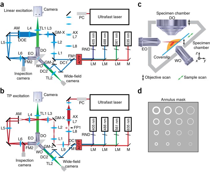
(a) CW laser sources at 405 nm, 488 nm, 561 nm and 635 nm are used for linear excitation. The four collimated laser beams are each expanded to a 1.5-mm diameter and then combined by using LaserMux dichroic mirrors (LM) into a single beam that is sent to the AOTF. Scanning galvo mirrors, GM-Z and GM-X; annulus mask (AM); the rear focal plane of excitation objective, EO; and a rear pupil inspection camera are conjugated with each other in sequence through relay lens L1 and L2 (45-mm and 90-mm focal length), L3 and L4 (50-mm and 150-mm focal length), L5 and L6 (125-mm and 125-mm focal length). DOE can be placed immediately in front of mask AM to generate an array of parallel Bessel beams. Detection objective, DO, is placed orthogonal to excitation objective EO. The emitted fluorescence is collected through DO and imaged onto the detection camera with tube lens TL1 (500-mm focal length). Flip mirror FM1 is used to divert the multicolor excitation to a separate wide-field imaging path that serves as a low-magnification view finder. Flip mirror FM2 is used to direct the annular excitation beam to the inspection camera. (b) A Chameleon ultrafast laser is used for TP excitation. A Pockels cell is used for laser intensity modulation, and the NIR beam is collimated and expanded to a 10-mm diameter. Axicon AX (0.5° cone angle) and lens L7 (100-mm focal length) are used to create an annular focus at focal plane FP1. This is then conjugated to GM-Z and all subsequent conjugation planes through relay lens L8 L9 (50-mm and 150-mm focal length). (c) Schematic of the specimen chamber, which consists of the chamber itself, excitation objective (EO), detection objective (DO), the specimen holder, and the wide-field view-finding objective. 3D images of the sample can be collected either by scanning the light sheet and DO in synchronization with one another, or by scanning the sample through the light sheet. (d) Mask AM contains an array of annuli array of differing outer and inner diameters to create Bessel beams of differing lengths and thicknesses. (This model and the associated mechanical drawings for custom components are available from HHMI after execution of a NDA.)
CW laser sources with excitation wavelengths at 405, 488, 561 and 635 nm are used for single-color and multicolor imaging via linear excitation. Each laser beam is collimated and expanded to a 1.5-mm beam diameter (1/e2) and then combined in a single co-linear beam before entering an AOTF (Supplementary Fig. 2a). The AOTF is used to select the currently active wavelengths and to control their amplitudes.
The output beam from the AOTF is sent to beam-scanning components (Supplementary Fig. 2b) that consist of two 3-mm-square scanning galvanometer (galvo) mirrors. The first, GM-Z, scans the virtual light sheet along the detection axis and is conjugated at 2× magnification to the second, GM-X, which scans the beam laterally to create the virtual light sheet. This second galvo is then conjugated at 3× magnification to an opaque mask AM (Fig. 3d) containing transmissive annuli of different maximum and minimum diameters defining different maximum and minimum NA for the eventual Bessel beam. This annulus mask is mounted on a 3D translational stage to allow accurate positioning and switching to different annular patterns. The annular beam emerging from mask AM is then conjugated to the rear focal plane of excitation objective EO.
If desired, a DOE can be placed in front of mask AM to generate an array of parallel excitation Bessel beams within the sample. However, because the individual beams from the DOE do not have similar phases, separation between the beams within the sample should be larger than the effective range of interaction between the side lobes of adjacent beams.
Detection objective DO, mounted on a detection objective piezo, is placed orthogonally to excitation objective EO (Supplementary Figs. 3a and 4). In the objective-scanning implementation, a 3D image stack is acquired by synchronizing the motion of the piezo to galvo GM-Z (black arrows, Fig. 3c) so that the excitation light sheet always overlaps with the detection focal plane. The emitted fluorescence is collected through the detection objective DO and imaged on the detection camera with a tube lens. The effective pixel size at the camera should be slightly smaller than the Nyquist limit of λdet/(4NAdet) to achieve the full theoretical resolution of the system.
In the TP modes, an ultrafast Ti-sapphire laser of tunable wavelength is used as the excitation source (Fig. 3b). The NIR laser beam passes through a Pockels cell for laser intensity modulation. To maximize the transmission laser power of the NIR laser beam through mask AM, NIR achromatic lens L7 and axicon AX are paired to create an annular ring of excitation at the front focal plane of lens L7 (ref. 26). This plane is conjugated to galvo GM-Z, and hence mask AM as well, at a magnification such that the dimensions of the excitation ring at AM match those of the chosen annulus. With this approach, more than 60% of the laser power can be transmitted through the annulus. A similar achromat/axicon subsystem can be placed between the AOTF and galvo GM-Z when more excitation energy is required for Bessel plane illumination with linear excitation.
The specimen chamber subassembly is shown schematically in Figure 3c and from the 3D model in Supplementary Figure 3a. The chamber itself (Supplementary Fig. 3b) has a vertical slot that is filled with the imaging buffer into which the specimen holder is inserted. There are also side ports for insertion of the excitation and detection objectives, as well as a third objective to provide an epifluorescence view of the sample to locate the region of interest during imaging. A piece of 0.1-mm-thick silicone plastic film is stretched over the sides of the excitation, detection and epi-illumination objectives and is clamped to the sides of the sample chamber to contain the medium in the sample chamber while still permitting the objectives to move with minimal resistance. A serpentine circulation channel is cut in the specimen chamber to allow heated water to flow in a separate circuit through the body of the chamber to keep the medium and the specimen at the desired temperature (e.g., 37 °C for live mammalian cell imaging).
All three objectives (EO, DO and WO) must be long-working-distance, water-immersion objectives. Owing to the physical size constraints between the excitation and detection objectives, the sum of the half-angles of their illumination cones must be less than 90°, and they must not mechanically intersect when orthogonal to one another and placed at a common focus (Supplementary Fig. 4). We have used two pairs of objectives (EO and DO) that satisfy these constraints. The first combination uses identical Nikon CFI Apo 40XW (0.8 NA, 3.5 mm WD) objectives as both the EO and DO, and the other uses a custom water immersion objective designed and built by Special Optics (0.65 NA, 3.74 mm WD) as the EO and a Nikon CFI Apo LWD 25XW (1.1 NA, 2 mm WD) as the DO. The 1.1-NA Nikon objective also has a correction collar that can be used to correct the spherical aberration induced by the refractive index differences of different imaging buffers and at different temperatures. Its axial resolution is also better matched to the transverse resolution of the 0.65-NA excitation lens, and its light collection ability is superior to the 0.8-NA configuration. Thus, the second objective combination is preferred.
The specimen holder (Supplementary Fig. 4) is mounted on a sample-scanning piezo that is mounted in turn on an xyz translational stage designed to position the sample region of interest to the volumetric region swept out by the Bessel beam. In the sample-scanning implementation, a 3D image stack is acquired by translating this piezo (green arrows, Fig. 3c), whereas the Bessel beam plane and detection objective remain stationary.
The microscope is controlled with a Supermicro SYS-7046GT-TRFP computer equipped with dual hexa-core processors (Xeon X5680) and 96 GB of RAM. The computer backplane contains seven PCIe slots and two PCI slots, providing enough space for the necessary control cards. Either an Andor IXon 885 EM-CCD camera or a Hamamatsu Orca-Flash 4.0 sCMOS camera is used for image detection. Collected images are written directly to a dual-disk array consisting of two SRS 7,200-r.p.m., 1-TB disks during imaging. Four-dimensional data stacks smaller than the RAM buffer can be stored in RAM and then downloaded to the drives later. Larger data arrays are best written directly to an external RAID array so that the ∼800 MB/s maximum recording rate of the Orca-Flash 4.0 sCMOS camera does not overload the typical ∼100 MB/s write speed of a single hard drive. An external RAID array also offers considerably greater storage space than a single drive, which can be easily filled in a couple of days of experiments. A NI PCIe-7852R multifunctional reconfigurable I/O board triggered by the imaging camera is used to generate control signal sequences through the connection box CA-1000 to synchronize the AOTF or Pockels cell, galvos and objective-or sample-scanning piezos with image collection. Analog control signals for the galvos and piezos are further conditioned by individual scaling amplifiers to better match the 16-bit resolution output of the FPGA card to the input signal range of each device. Customized control software was developed in Labview 2012 by Coleman Technologies, and it includes routines for microscope calibration and operation under different imaging modes, as well as tools for reviewing the collected data in situ. This software is also available from HHMI upon execution of an NDA. Typical control signal sequences for the various operational modes of Bessel beam plane illumination are shown in Figure 4.
Figure 4: Control signal sequences for Bessel beam plane illumination. 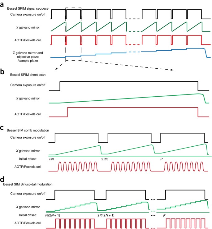
(a) General control signal sequences for 3D imaging. Control signals for the AOTF/Pockels cell, galvos GM-X and GM-Z, the detection-objective piezo and the sample-scan piezo are triggered by the imaging camera. (b) Control signal sequences for the sheet-scan mode at each image plane. (c) Control signal sequences for the SIM mode with sinusoidal modulation at each image plane. (d) Control signal sequences for the SIM mode with comb modulation at each image plane. Phase shifting of the illumination pattern is realized by changing the initial position of the excitation beam.


Scanning mode
-
The volumetric image of the sample can be obtained either by objective scan or sample scan. In objective-scan mode, both the detection objective and the excitation light sheet are scanned across the sample simultaneously while a stack of images are collected sequentially during scanning at different axial positions. Objective-scan mode is suited for imaging samples with similar dimensions in all directions, e.g., C. elegans embryo. In contrast, sample scanning can be used to image thin samples, as the excitation beam can be much shorter than that in the objective-scan mode. This substantially reduces the excitation beam side lobes. In sample-scan mode, the excitation light sheet and the detection objective are fixed while the sample is scanned across the light sheet for 3D imaging (Fig. 3c). The data analysis is slightly different for raw data collected by the two operation modes.
Procedure
Collimate and combine CW laser beams
Timing ∼10 h
Critical Step
The alignment of the Bessel beam plane illumination microscope should comply with general rules and laser safety regulations for optical system alignment. Special care should be taken while aligning the NIR beam for TP excitation.
Critical Step
The system should be aligned at ambient temperature, which should fall in the range of 20–25 °C. The actual temperature variation should be less than 1 °C; variation in temperature causes substantial focal length drifting of the microscope objectives.
Critical Step
Initial alignment (Steps 1–23) needs to be performed only for the initial construction of the microscope; commence subsequent imaging experiments at Step 24.
-
1
Collimate each beam by using its specific beam-expanding components so that all beams have a common beam diameter. Combine all CW laser beams into a single coincident beam before the AOTF. Align the rest of the microscope by using the 488-nm CW laser; the system is then aligned for other CW lasers automatically because they share the same optical path.
Conjugate galvos GM-X, GM-Z, annulus mask and excitation objective
Timing 10–20 h
Critical Step
The correct conjugation of the galvos to each other as well as the annulus mask AM and the rear pupil of the excitation objective EO is critical to ensure that the beam only translates in x and z within the sample and does not also tilt as the galvos are scanned. Each plane is conjugated to the next by using a pair of relay lenses in a 2f1 + 2f2 configuration.
-
2
With galvos GM-Z and GM-X powered at their mid-range control voltages, rotate GM-Z about its axis until the light beam from GM-Z is centered on GM-X, and the light beam from GM-X is orthogonal to mask AM.
-
3
Conjugate GM-Z to GM-X by placing an inspection camera at the plane of GM-X, while modulating the angle of GM-Z at a few Hertz. Iteratively adjust the axial positions of the two relay lenses until the mirror of GM-Z is in focus and does not wobble when viewed through the inspection camera.
-
4
Place the inspection camera at the plane of mask AM, and repeat the procedure described in Step 3 until the mirror of GM-X is in focus and is not wobbling at the plane of AM.
-
5
As a final check, place mask AM at this second conjugation plane, and center an annulus that will eventually produce a Bessel beam of ∼600 nm in diameter and 30 μm in length (e.g., NAOD = 0.4 and NAID = 0.36, where OD is outer diameter and ID is inner diameter) in the sample on the impinging laser beam. Move the inspection camera to the side of AM opposite the galvos, and then image the illuminated annulus onto the camera. Adjust the relay lenses if necessary to ensure that the illumination through the annulus does not vary as the galvo tilts are modulated.
-
6
Conjugate annulus mask AM to excitation objective EO. The specimen chamber should be designed with a small beam exit window opposite objective EO, along its axis. Fill the chamber with water, and view the annulus of light emerging from the window on a white screen a minimum of 50 cm away. Place a mark on the screen at the point where the axis of EO intersects the screen. Center the annular beam in the rear pupil of EO by translating the x and y right-angle prism mirrors immediately before EO until the annular beam on the screen is centered with respect to the marked reference point. Adjust the axial position of EO until the image of the annulus is in focus on the screen. This completes the initial centering and conjugation of the beam relative to EO.
Align the detection path
Timing 10–20 h
-
7
Align the detection objective DO. Fill the specimen chamber with the prepared Alexa Fluor 488 hydrazide solution and move mask AM laterally to the position of a round aperture (not an annulus) that produces a Gaussian beam of at least 0.3 NA in the chamber. Set the output of the 488-nm laser to maximum, set galvos GM-Z and GM-X at their mid-range positions, set the detection objective piezo to its mid-range position and remove detection tube lens TL1. Place a white screen at a minimum of 50 cm from the rear pupil of objective DO and place a mark on the screen at the point where the axis of DO intersects the screen. Adjust the axial position of DO until the beam of fluorescence emission emerging from DO is collimated. Adjust the lateral position of DO until the beam emerging from DO is centered with respect to the marked reference point.
-
8
Align the tube lens TL1. Remount tube lens TL1. Move mask AM laterally back to the position that produces a Bessel beam of ∼600 nm diameter and 30 μm length in the chamber. Adjust the axial position of TL1 until the image of the Bessel beam is in focus on the detection camera. Adjust the lateral position of TL1 until the image of the beam is centered in the field of view of the camera.
-
9
Fine-tune the annular beam centration in the rear pupil of EO. With a Bessel beam excited in the AF 488 solution and the galvos and piezo for DO all at mid-range, measure the width of the Bessel beam on the detection camera at two axial locations symmetric about its center. Adjust the position of the annular beam entering objective EO along the z axis with the appropriate right angle prism just before EO until the beam widths at both locations are the same (Fig. 5 shows an unaligned case in which only one end of the beam is in focus). Adjust the position of the annular beam along the x axis until the image of the Bessel beam is parallel to the x axis on the detection camera (Fig. 5a shows an unaligned case in which the beam is not parallel to the x axis).
Figure 5: Microscope alignment. 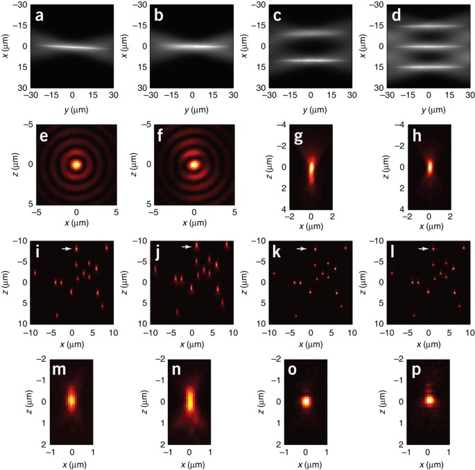
(a) An unaligned Bessel beam tilted in the xy plane. (b) An unaligned Bessel beam tilted in xy plane. The right side of the beam is in focus, but the left side is not. (c) A Bessel beam that, when swept in the x direction, does not remain in focus, so that the virtual light sheet and the detection focal plane are not coincident. (d) An aligned Bessel beam that is in focus at all x positions across the scan plane. (e) The cross-sectional intensity profile of a properly aligned Bessel beam. (f) The cross-sectional intensity profile of a Bessel beam caused by nonuniform illumination across the annular ring and mis-conjugation of the the annular ring to the rear pupil of excitation objective EO. (g) The detection wide-field xz PSF with strong spherical aberration. (h) The detection wide-field xz PSF after aberration correction with the correction collar of DO. (i) xz MIP view of a field of fluorescent beads imaged in the sheet-scan mode showing symmetric PSFs in the axial direction across the entire field of view. (j) xz MIP view of a field of fluorescent beads imaged in the sheet-scan mode, with a 1 μm offset between the center of the light sheet and the focal plane of DO, showing an identical axial asymmetry in the PSF across the entire field of view. (k) Same as in i, except acquired in the OS-SIM mode with N = 7 phases. Note the substantially tighter PSF in the axial direction. (l) Same as in j, except acquired in the OS-SIM mode with N = 7 phases, and a 0.3 μm offset between the excitation and detection planes. (m–p) Zoomed-in view of the same fluorescent bead marked in i–l. In general, the SIM modes require an even tighter axial alignment than the swept-sheet modes.

Fine-tuning
Timing 10–20 h
-
10
Fine-tune the conjugation to EO. Move the detection objective piezo to the top of the desired z-scan range. Adjust the control voltage of galvo GM-Z until the center of the Bessel beam is in focus at this new position, as determined by a minimum cross-sectional width midway along its length, as measured by the control utility. Repeat this process with the piezo moved to the bottom of the desired z-scan range. Adjust the axial positions of the relay lenses between mask AM and objective EO until the beam is in focus along its entire length at both the top and the bottom extremes of the z field of view.
-
11
Calibrate the galvos. Move the detection objective piezo in 10-μm steps from −40 to 40 μm. At each position, adjust the control voltage to galvo GM-Z until the Bessel beam is back in focus. Apply linear regression to the galvo voltage versus the objective position measurements to determine the calibration constant of z beam displacement per volt applied to the galvo. The correlation coefficient should be at least 0.999 for the Bessel beam to remain at the focal plane of DO across the entire z field of view. Next, adjust the control voltage to galvo GM-X in approximately ten equal steps of amplitude such that the beam moves across the entire x field of view as seen on the detection camera. Use the camera images to determine the beam position for each control voltage and apply linear regression to determine the calibration constant of x beam displacement per volt applied to the galvo.
-
12
Confirm conjugation and centration. Confirm that the light sheet swept by the Bessel beam remains in focus across the entire xy field of view, for all z planes of the desired 3D stack (Fig. 5c shows a case where the beam is not in focus at all x positions in a given plane, Fig. 5d shows the case of correct alignment). Repeat Steps 2–6 and 9 and 10 as needed to achieve these conditions. This completes the alignment of the linear excitation beam.
-
13
Mount the rear pupil inspection camera. Mount the camera at the location specified in Figure 3a and, with the flip mirror in the up position, adjust the camera position so that the annular light ring is in focus (i.e., conjugate to mask AM and the rear pupil of objective EO) and centered in the field of view. Record and save the image of the annulus. Subsequent alignment of the system, if necessary, can be accomplished by adjusting the position, focus and conjugation (i.e., no wobble or intensity variation under scanning) of the excitation path as described in Steps 2–6 to match this stored image.
System characterization
Timing 10–20 h
-
14
Fine-tune and measure the wide-field detection PSF. Flush the Alexa Fluor 488 solution from the imaging chamber with water until no fluorescence can be observed on the detection camera. Fill the imaging chamber with water. Place the prepared fluorescent bead sample on the specimen holder. Translate the bead sample to the center of the imaging field. Position a single isolated bead within the Bessel beam. Use the program utility to measure the 3D detection PSF. This works by leaving the x galvo fixed, while moving the z galvo and detection objective piezo together to acquire a 3D image stack of the bead. Check the xz view of this stack for any asymmetry in the axial PSF (Fig. 5g). Adjust the correction collar of DO to achieve axial symmetry. If the range of the collar is insufficient, return the collar to its mid-range position, and iterate in slight axial moves of objective DO and tube lens TL1 until axial symmetry is achieved (Fig. 5h). Check the xz and yz views of the 3D stack for lateral asymmetry in the PSF. Iteratively adjust the lateral positions of objective DO and tube lens TL1 until symmetry is achieved, while maintaining the image of the bead in approximately the same position on the camera. Record the final, symmetric 3D detection PSF for eventual use in reconstruction of SR-SIM mode data, making sure that the signal from only the desired target bead appears in the PSF data.
-
15
Characterize the Bessel beam cross-sectional intensity. Position an isolated fluorescent bead in focus at the common center of the imaging field and the Bessel beam by using the sample translational stages. Use the program utility to measure the cross-section of the Bessel beam. This works by using the galvos to raster-scan the excitation beam in 100-nm steps across the bead over a ±5-μm range in the xz plane while recording an image at each position. The integrated fluorescence recorded from the bead in each image gives a measure of the intensity of the beam at the associated xz position. The image created by the entire xz set of these measurements yields the cross-section of the Bessel beam. The image should closely approximate an ideal Bessel beam, with symmetric side lobes (Fig. 5e). If not (e.g., Fig. 5f), check with the rear pupil inspection camera that the intensity is uniform across the annulus, and that both intensity and position of the annulus remain constant as the galvos are scanned. Retune the conjugation of all elements and centration of the annular beam as described in Steps 2–6 until a symmetric Bessel beam is achieved.
-
16
Characterize the Bessel swept-sheet PSF. Position a field of fluorescent beads within the volume to be imaged. Take a 3D image stack of this field in the swept-sheet mode across an image volume of ∼50 × 50 × 50 μm. The 3D image of each fluorescent bead within the field corresponds to the Bessel sheet-scan PSF at the bead position. All PSFs should be identical and symmetric in the axial direction across the entire imaging field (Fig. 5i), although they may be less intense at the edges of the field in the y direction owing to finite extent of the beam. Adjust the initial offset of the detection objective piezo to achieve symmetry if the PSFs are uniformly asymmetric in the same axial direction. Return to Steps 10–12 if the PSFs are not uniform or are asymmetric in different directions. Record the image of an isolated bead taken in the swept sheet mode for eventual use as the reference 3D PSF in deconvolution of image data.
-
17
Characterize the Bessel OS-SIM PSF. Take a 3D image stack of a field of fluorescent beads with the Bessel OS-SIM mode with a periodic pattern having H = 3 or 4 harmonics, requiring N = 7 or 9 images per plane. Reconstruct the final 3D stack from the raw data by using the OS-SIM algorithm. The 3D image of each fluorescent bead within the field corresponds to the Bessel OS-SIM PSF at the bead position. If the xz PSFs are uniformly asymmetric axially (Fig. 5l), adjust the offset position of the detection objective piezo until symmetry is achieved (Fig. 5k). Return to Steps 10–12 if the PSFs are not uniform or asymmetric in different directions. The axial resolution of the reconstructed OS-SIM image (Fig. 5k) should be substantially better than that taken by the Bessel swept-sheet mode (Fig. 5k). Record the image of an isolated bead taken in the OS-SIM mode for eventual use as the reference 3D PSF in deconvolution of image data. This completes the system alignment for linear excitation with a single Bessel beam.
(Optional) Bessel beam array alignment
Timing 1–2 h
-
18
Create an array of parallel Bessel beams. Parallel Bessel beams can be used, if desired, to increase the speed of Bessel plane SIM and/or to reduce phototoxicity by reducing the peak intensity within the sample. Place diffractive optical element DOE against the annulus mask on the side facing the galvos to create multiple excitation beams simultaneously.
-
19
Check the DOE alignment and beam spacing. Fill the imaging chamber with Alexa Fluor 488 dye solution. Rotate the DOE around its axis until all of the parallel excitation beams are in focus simultaneously (Fig. 5d). Check that the fan angle of the DOE is large enough so that the side lobes of adjacent beams do not interfere. Return to Step 12 and repeat other alignment steps as needed.
-
20
Select the beam spacing for Bessel SIM modes. Use the image of the parallel beams in dye solution to measure the exact spacing between beams. For the OS-SIM and SR-SIM modes, make sure that period T of the written SIM grating pattern is given by the beam spacing divided by an integer.
(Optional; for TP Bessel beam plane illumination and TP Bessel SIM mode) TP mode alignment
Timing 5–10 h
-
21
Create an excitation annulus for TP imaging. Adjust the Chameleon laser source to a visible wavelength (e.g., 770 nm). Attenuate the beam power by using a half-wave plate and a polarizer. Align the Pockels cell according to the Pockels cell alignment manual. Collimate and expand the NIR beam to an ∼10-mm beam diameter. Place another inspection camera at the focal plane FP1 (Fig. 3b) of lens L7. An annular focus created by axicon AX and lens L7 should be visible. Adjust the input beam centration and perpendicularity to AX until the intensity is uniform across the annular beam.
-
22
Perform initial conjugation and alignment of the annular beam. Remove this secondary inspection camera. Insert lens L9 into the optical path and conjugate the annular focus first to galvo mirror GM-Z. Tune the Chameleon laser to the desired NIR wavelength for TP excitation. Adjust the axial positions of relay lenses L8 and L9 until the annular beam is in focus at galvo GM-Z. Adjust the lateral positions of L8 and L9 as well as the tilt angle of dichroic mirror DC1 until the annular beam passes through the desired annulus in mask AM. View the filtered annular beam on the rear pupil inspection camera from Step 13. Again adjust L8, L9 and DC1 until the intensity of the annular beam is uniform.
-
23
Fine-tune conjugation and alignment. The differences in the focal lengths at visible and NIR wavelengths of all relay lenses in the optical path may cause the GM-Z, GM-X, AM and the rear pupil of objective EO to no longer be mutually conjugated. Test the conjugation of these elements and centration to the rear pupil of EO by using the same procedures as those given above for linear excitation. Confirm with an isolated fluorescent bead the uniformity of the scanned TP light sheet. Confirm with a field of beads the uniformity, symmetry and quality of the overall 3D PSF in the TP swept-sheet and SIM modes. Record the image of an isolated bead taken in the TP swept-sheet mode for eventual use as the reference 3D PSF in deconvolution of image data.
Image acquisition
Timing 0.5–1 h
Critical Step
We have provided guidelines below for a typical experiment. We do not describe sample preparation, as this will be the same as for conventional wide-field and confocal fluorescence microscopy. The sample mounting method will be dictated by the instrument design. Examples of sample preparation and mounting can be found in previous publications10,17.
-
24
Estimate the desired excitation beam length and thickness on the basis of the sample size, desired spatial resolution, acquisition mode (objective scan or sample scan), imaging speed, number of time points and sample brightness. Use Table 2 to select an appropriate annulus on the mask on the basis of this estimation. Select the beam that is just long enough to cover the imaging field of interest and thin enough to give the desired spatial resolution in order to minimize the influence of the Bessel beam side lobe.
Table 2 Approximate Bessel beam length and FWHM of the central peak for selected annuli with different illumination NAOD and NAID values. -
25
Fill the imaging chamber with the corresponding dye solution. Verify the Bessel beam alignment as in Step 9.
-
26
Fill the sample chamber with the desired imaging buffer. Characterize the system PSF again as described in Steps 15–17.
-
27
The system is ready for room temperature imaging. If room temperature is compatible with the sample, load the sample and then proceed to Step 32 below. For imaging at elevated temperature (e.g., 37 °C), first perform Steps 28–32.
-
28
Use a water bath to heat a reservoir of water. Turn on the water pump to circulate the heated water through the channels in the walls of the sample chamber.
-
29
Place a sample with a field of fluorescent beads in the chamber. Monitor the temperature of the imaging buffer in the chamber and periodically image the field of beads in the swept-sheet or OS-SIM modes as the temperature rises. Adjust the initial offset of the detection objective piezo and the correction collar of DO to maintain a symmetric, aberration-free axial PSF from the beads.
-
30
Adjust the temperature of the water bath as needed and repeat Step 29 periodically until the buffer in the chamber equilibrates at the desired imaging temperature.
-
31
Replace the imaging buffer in the chamber with fresh buffer, prewarmed to the desired equilibrium temperature if you are not imaging at room temperature. The system is now ready for imaging.
-
32
During imaging, it is crucial to keep the excitation light sheet centered on the focal plane of objective DO to achieve the desired performance, especially for Bessel SIM. Both of the following two methods can be used to ensure that the excitation light sheet remains in focus.
-
A
Maximize the in-focus modulation depth
-
i
Occasionally apply a fixed, periodic modulation pattern, such as that required for SIM, and adjust the offset of the detection objective piezo until the maximum modulation depth is observed.
-
i
-
B
Maximize the SNR of OS-SIM reconstructed results
-
i
Occasionally acquire an image of the sample in OS-SIM mode and adjust the piezo offset until the SNR of the OS-SIM reconstruction is a maximum. The OS-SIM reconstruction depends only on the fundamental modulation harmonic of the illumination pattern whose amplitude is maximum when the modulation pattern is in focus.
-
i
-
A
Data processing
Timing variable; ∼1–3 min per image volume
-
33
Analyze the data by using either option A, B or C, depending on how the data were acquired. Note that for option C, the raw 3D data stack with N images per plane of N different phases of the applied grating are analyzed by using the algorithm originally developed for wide-field 3D-SIM. A thorough description with more details is available elsewhere14.
-
A
Data obtained in linear or TP swept-sheet modes with an objective scan
-
i
Measure the system PSF by using the corresponding imaging method as described in Step 16. The PSF must be measured on a single, isolated fluorescent bead at voxel sizes that are smaller in all three dimensions than half the theoretical resolution limit.
-
ii
Subtract the noise background from the measured PSF data volume.
-
iii
Deconvolve the acquired data by using the Richardson-Lucy 3D deconvolution algorithm in MATLAB and the processed PSF.
-
i
-
B
Data obtained in linear or TP swept-sheet modes with a sample scan
-
i
Measure the system PSF as described in Step 33A(i).
-
ii
Process the measured PSF as described in Step 33A(ii).
-
iii
Transform the data from the skewed scanning coordinates back to the optical xyz coordinates.
-
iv
Deconvolve the transformed data as described in Step 33A(iii).
-
i
-
C
Data obtained in SR-SIM mode
-
i
Pre-process the original images by using flat-field correction and soften the image edges.
-
ii
Separate the spectral information components. As discussed above, the raw data consist of three or more different information components that are originally located at different positions in frequency space, and need to be separated first. The raw data, including a total of 2N + 1 images per image plane, can be formulated as a linear combination of the information components in frequency space and information components need to be calculated from the raw images.
-
iii
Measure the system PSF to acquire the effective OTF of each information component, Om. This is done by acquiring a Bessel SIM data set on a single fluorescent bead under exactly the same experimental conditions as the data to be reconstructed. The voxel size of both the PSF and the raw data must be smaller than the Nyquist limit.
-
iv
Apply an inverse filter and reassemble each information component back to its appropriate location in frequency space. Transform back to real space to produce the final reconstructed image with extended resolution.
-
i
-
A
Troubleshooting
Troubleshooting advice can be found in Table 3.
Timing
Step 1, collimate and combine CW laser beams: ∼10 h
Steps 2–6, conjugate galvos GM-X, GM-Z, annulus mask and excitation objective: 10–20 h
Steps 7–9, align the detection path: 10–20 h
Steps 10–13, fine-tuning: 10–20 h
Steps 14–17, system characterization: 10–20 h
Steps 18–20, (optional) Bessel beam array alignment: 1–2 h
Steps 21–23, (optional) TP mode alignment: 5–10 h (Steps 21–23 only need to be performed for TP Bessel beam plane illumination and TP Bessel SIM mode)
Steps 24–32, image acquisition: 0.5–1 h
Step 33, data processing: variable; ∼1–3 min per image volume, depending on the image data size and the computation power of the data-processing computer
Anticipated results
Figure 6 shows the xy and xz maximum intensity projection (MIP) views of fluorescently labeled microtubules in a fixed LLC-PK1 cell, imaged with the SR-SIM mode in PBS. An annular illumination pattern of NAOD = 0.59, NAID = 0.55 was used, yielding a Bessel beam of ∼410 nm in central peak thickness and ∼15 μm in length. This represents a relatively high NA yet a short beam for Bessel beam plane illumination. Both of these attributes are desirable, as long as they are consistent with the requirements of the sample. High NA yields high spatial frequencies for higher resolution SIM reconstruction and short beam length results in low side lobe energy and thus less out-of-focus background, which can otherwise compromise the SNR in SIM reconstructions. For the case of the thin cultured cell in Figure 6a,b, these parameters work well because a 15-μm beam is sufficient to cover the ∼10-μm thickness of the cell in sample-scan mode, and because the cell is so thin that even at high NA the sample-induced aberrations are negligible.

(a,b) xy and xz MIP views of a fixed LLC-PK1 cell with fluorescently labeled microtubules imaged in the SR-SIM mode by using nine phases and comb modulation. (c,d) Magnified views of the boxed regions in a and b. (e) Line width measurements from the microtubules c and d in the x, y and z directions. (f) A raw image during the acquisition with comb modulation, with arrows showing the maxima of the grating pattern within the sample. (g) Magnified view of the boxed region in f. (h,i) xy and xz MIP views of a Dictyostelium discoideum cell imaged in the SR-SIM mode with sinusoidal modulation. (j) A raw image frame during the acquisition, with arrows showing the very weak modulation pattern produced by sinusoidal modulation. (k) MIP view of the real-time, in-situ OS-SIM reconstruction from the sine mode data that can be used to indicate whether the modulation amplitude and excitation power are sufficient to obtain a good SR-SIM reconstruction. (l,m) xy and xz MIP views of a C. elegans embryo imaged by using the SR-SIM mode with five phases and comb modulation. (n) A raw image ∼15 μm below the sample surface, with arrows showing the maxima of the comb pattern. Note that the pattern is stronger on the left side than on the right, as optical aberrations and scattering cause distortions in the pattern as the beam prorogates from left to right. (o) xy MIP of the real-time, in-situ OS-SIM reconstruction used for visual feedback during acquisition. Note that the OS-SIM reconstruction has both lower x resolution and lower SNR than the final SR-SIM reconstruction in l. Scale bars, 5 μm (a,b,f,h,l), 1 μm (c,d,g).
A comb pattern of 1.8 μm period, visible in the raw data frame in Figure 6f,g, was used to create the grating pattern for SIM. At NAOD = 0.59, this required acquisition of N = 9 phase-stepped images per plane for the 3D SIM reconstruction. The entire raw data stack is shown in Supplementary Video 1. A large number of phases N improves the SNR of the final reconstruction, because it makes use of more information and includes low frequency harmonics of higher amplitude. It does, however, take longer to acquire and expends more of the limited photobleaching-dictated photon budget. Fortunately, for fixed samples such as those shown here, these are not important concerns.
With these imaging conditions, the theoretical spatial resolution in Figure 6a,b is ∼160 nm in the x direction, ∼240 nm in y and ∼290 nm in z. These predictions are consistent with the experimental results (Fig. 6e).
Figure 6h,i shows MIP views of a living Dictyostelium discoideum cell expressing F-actin (labeled by GFP), imaged by using the SR-SIM mode with sinusoidal modulation. This modulation pattern was chosen because it requires the minimum N = 3 images per plane required for SIM reconstruction, and hence is more compatible with rapid and noninvasive imaging of quickly moving, light-sensitive specimens such as these. An illumination annulus of NAOD = 0.43, NAID = 0.4 was chosen to create a longer Bessel beam in order to cover the potential migration of the cell over the course of the imaging. A comparatively long modulation period of 3.5 μm was used to improve the optical sectioning capability. Although this still results in near-optimal axial resolution improvement to ∼350 nm in the SIM reconstruction, the lateral resolution improvement beyond the ∼240-nm limit of diffraction is negligible.
One limitation of using sinusoidal modulation for Bessel plane SR-SIM is that the ratio of the amplitude of the fundamental harmonic to the DC harmonic is typically much smaller (e.g., Fig. 6j and Supplementary Video 2) than that with the comb function, thus requiring a higher SNR in the raw data to get a satisfactory reconstruction. As a quick check to see whether the SNR of the raw data is sufficient, a trial 3D stack can be collected and analyzed in situ with the OS-SIM algorithm (Fig. 6k) and the power adjusted accordingly just before the desired 4D data set is collected.
Multicellular specimens typically require longer and thicker Bessel beams, both to span the complete specimen and to reduce the sensitivity to sample-induced aberrations, which are a much greater concern in such specimens. For example, the live C. elegans embryo in Figure 6m was imaged with a five-phase Bessel plane SR-SIM with comb modulation at NAOD = 0.31 and NAID = 0.27. This produced a Bessel beam ∼40 μm long, which was sufficient to image the ∼60 × 35 μm embryo, provided that the short axis of the specimen was aligned parallel to the beam. In general, all asymmetric specimens should be mounted with their short axes parallel to the beam, to permit the shortest possible beam to be used with the least possible amount of energy in the side lobes. To cover the scan of the long axis more quickly and to reduce photodamage, a DOE was added producing seven parallel Bessel beams. A SIM pattern period of 2.12 μm was chosen to ensure the strength of the fundamental modulation order. The theoretical spatial resolution is ∼200 nm in the x direction, ∼240 nm in y and ∼430 nm in z. As above, the OS-SIM algorithm can be used (Fig. 6o) to verify that modulation amplitude and excitation power are sufficient to yield good-quality SR-SIM reconstructions; it can be very difficult to know this from the raw images directly (Fig. 6n and Supplementary Video 3).
References
Siedentopf, H. & Zsigmondy, R. Über Sichtbarmachung und Groessenbestimmung ultramikroskopischer Teilchen, mit besonderer Anwendung auf Goldrubinglaesern. Ann. d. Physik 10, 1–39 (1903).
Huisken, J., Swoger, J., Del Bene, F., Wittbrodt, J. & Stelzer, E.H.K. Optical sectioning deep inside live embryos by selective plane illumination microscopy. Science 305, 1007–1009 (2004).
Greger, K., Swoger, J. & Stelzer, E.H.K. Basic building units and properties of a fluorescence single plane illumination microscope. Rev. Sci. Instrum. 78, 023705 (2007).
Keller, P.J., Schmidt, A.D., Wittbrodt, J. & Stelzer, E.H.K. Reconstruction of zebrafish early embryonic development by scanned light-sheet microscopy. Science 322, 1065–1069 (2008).
Tomer, R., Khairy, K., Amat, F. & Keller, P.J. Quantitative high-speed imaging of entire developing embryos with simultaneous multiview light-sheet microscopy. Nat. Methods 9, 755–763 (2012).
Krzic, U., Gunther, S., Saunders, T.E., Streichan, S.J. & Hufnagel, L. Multiview light-sheet microscope for rapid in toto imaging. Nat. Methods 9, 730–733 (2012).
Ahrens, M.B., Orger, M.B., Robson, D.N., Li, J.M. & Keller, P.J. Whole-brain functional imaging at cellular resolution using light-sheet microscopy. Nat. Methods 10, 413–420 (2013).
Keller, P.J. Imaging morphogenesis: technological advances and biological insights. Science 340, 1234168 (2013).
Keller, P.J. et al. Fast, high-contrast imaging of animal development with scanned light-sheet–based structured-illumination microscopy. Nat. Methods 7, 637–642 (2010).
Planchon, T.A. et al. Rapid three-dimensional isotropic imaging of living cells using Bessel beam plane illumination. Nat. Methods 8, 417–423 (2011).
Durnin, J., Miceli, J.J. & Eberly, J.H. Comparison of Bessel and Gaussian beams. Opt. Lett. 13, 79–80 (1988).
Truong, T.V., Supatto, W., Koos, D.S., Choi, J.M. & Fraser, S.E. Deep and fast live imaging with two-photon scanned light-sheet microscopy. Nat. Methods 8, 757–760 (2011).
Neil, M.A.A., Juškaitis, R. & Wilson, T. Method of obtaining optical sectioning by using structured light in a conventional microscope. Opt. Lett. 22, 1905–1907 (1997).
Gustafsson, M.G. Surpassing the lateral resolution limit by a factor of two using structured illumination microscopy. J. Microsc. 198, 82–87 (2000).
Gustafsson, M.G.L. et al. Three-dimensional resolution doubling in wide-field fluorescence microscopy by structured illumination. Biophys. J. 94, 4957–4970 (2008).
Shao, L., Kner, P., Rego, E.H. & Gustafsson, M.G.L. Super-resolution 3D microscopy of live whole cells using structured illumination. Nat. Methods 8, 1044–1046 (2011).
Gao, L. et al. Noninvasive imaging beyond the diffraction limit of 3D dynamics in thickly fluorescent specimens. Cell 151, 1370–1385 (2012).
Roh-Johnson, M. et al. Triggering a cell shape change by exploiting preexisting actomyosin contractions. Science 335, 1232–1235 (2012).
Habib, S.J. et al. A localized Wnt signal orients asymmetric stem cell division in vitro. Science 339, 1445–1448 (2013).
Majoul, I.V. et al. Fast structural responses of gap junction membrane domains to AB5 toxins. Proc. Natl. Acad. Sci. USA 110, E4125–4133 (2013).
Schermelleh, L., Heintzmann, R. & Leonhardt, H. A guide to super-resolution fluorescence microscopy. J. Cell Biol. 190, 165–175 (2010).
Cella Zanacchi, F. et al. Live-cell 3D super-resolution imaging in thick biological samples. Nat. Methods 8, 1047–1049 (2011).
Cella Zanacchi, F., Lavagnino, Z., Faretta, M., Furia, L. & Diaspro, A. Light-sheet confined super-resolution using two-photon photoactivation. PLoS ONE 8, e67667 (2013).
Friedrich, M., Gan, Q., Ermolayev, V. & Harms, G.S. STED-SPIM: stimulated emission depletion improves sheet illumination microscopy resolution. Biophys. J. 100, L43–L45 (2011).
Fahrbach, F.O., Simon, P. & Rohrbach, A. Microscopy with self-reconstruction beams. Nat. Photon. 4, 780–785 (2010).
Bélanger, P.A. & Rioux, M. Ring pattern of a lens-axicon doublet illuminated by a Gaussian beam. Appl. Opt. 17, 1080–1088 (1978).
Acknowledgements
We thank T. Planchon for help with the instrument; H. White and S. Michale for cell culture, transfection and staining; and we thank D. Milkie of Coleman Technologies for custom instrument control software. L.G. acknowledges the support of a Stony Brook University start-up grant.
Author information
Authors and Affiliations
Contributions
L.G. and E.B. conceived the project and designed the experiments; L.G. and B.-C.C. performed experiments; L.G. and L.S. analyzed the data; and L.G. and E.B. wrote the paper with the input of all other authors.
Corresponding author
Ethics declarations
Competing interests
US patent application no. US20110304723 A1, assigned to the Howard Hughes Medical Institute, covers a number of aspects concerning Bessel beam plane illumination microscopy.
Integrated supplementary information
Supplementary Figure 1 3D opto-mechanical model of the Bessel beam plane illumination microscope, with dashed boxes outlining its functional sub-assemblies.
(a) Top-down view of the microscope. (b) Tilted view of the microscope. (This model and the associated mechanical drawings for custom components are available from HHMI after execution of a non-disclosure agreement (NDA).)
Supplementary Figure 2 Bessel beam plane illumination microscope sub-assembly.
(a) Magnified view of the laser combination sub-assembly. The optical path of each laser beam includes an ND filter, a beam expander used to bring the beam to a diameter common with all others, and a four-axis beam steering assembly used to attain perfect overlap of all the beams. (b) Magnified view of the beam scanning and annular beam shaping sub-assembly.
Supplementary Figure 3 Bessel beam plane illumination microscope sub-assembly.
(a) Magnified view of the specimen chamber sub-assembly, the heart of the microscope. (b) Magnified view of the specimen chamber alone, showing objective ports and water channels for maintaining the desired temperature.
Supplementary information
3D opto-mechanical model of the Bessel beam plane illumination microscope, with dashed boxes outlining its functional sub-assemblies.
(a) Top-down view of the microscope. (b) Tilted view of the microscope. (This model and the associated mechanical drawings for custom components are available from HHMI after execution of a non-disclosure agreement (NDA).) (PDF 280 kb)
Bessel beam plane illumination microscope sub-assembly.
(a) Magnified view of the laser combination sub-assembly. The optical path of each laser beam includes an ND filter, a beam expander used to bring the beam to a diameter common with all others, and a four-axis beam steering assembly used to attain perfect overlap of all the beams. (b) Magnified view of the beam scanning and annular beam shaping sub-assembly. (PDF 375 kb)
Bessel beam plane illumination microscope sub-assembly.
(a) Magnified view of the specimen chamber sub-assembly, the heart of the microscope. (b) Magnified view of the specimen chamber alone, showing objective ports and water channels for maintaining the desired temperature. (PDF 269 kb)
Two views of the relative positions of excitation objective EO, detection objective DO, the widefield viewfinding objective, the sample coverslip, and the sample holder.
(a)Tilted view. (b) Top-down view. (PDF 247 kb)
Supplementary Video 1
Raw image stack of a fixed LLC-PK1 cell with fluorescently labeled microtubules imaged in the SR-SIM mode with nine phases comb modulation. (AVI 12325 kb)
Supplementary Video 2
Raw image stack of a Dictyostelium discoideum cell imaged in the SR-SIM mode with sinusoidal modulation. (AVI 1512 kb)
Supplementary Video 3
Raw image stack of a C. elegans embryo imaged in the SR-SIM mode with five phases comb modulation. (AVI 25503 kb)
Rights and permissions
About this article
Cite this article
Gao, L., Shao, L., Chen, BC. et al. 3D live fluorescence imaging of cellular dynamics using Bessel beam plane illumination microscopy. Nat Protoc 9, 1083–1101 (2014). https://doi.org/10.1038/nprot.2014.087
Published:
Issue Date:
DOI: https://doi.org/10.1038/nprot.2014.087
This article is cited by
-
Bessel light beam for a surgical laser focusing telescope—a novel approach
Lasers in Medical Science (2024)
-
Optical-resolution photoacoustic microscopy with a needle-shaped beam
Nature Photonics (2023)
-
Mastering lanthanide energy states for next-gen photonic innovation
Science China Chemistry (2023)
-
Generation of multiple focal pattern via phase modulated radial and azimuthal variant vector beam
Optical and Quantum Electronics (2023)
-
Capturing the start point of the virus–cell interaction with high-speed 3D single-virus tracking
Nature Methods (2022)
Comments
By submitting a comment you agree to abide by our Terms and Community Guidelines. If you find something abusive or that does not comply with our terms or guidelines please flag it as inappropriate.
