
Abstract
The initial phase of malaria infection is the pre-erythrocytic phase, which begins when parasites are injected by the mosquito into the dermis and ends when parasites are released from hepatocytes into the blood. We present here a protocol for the in vivo imaging of GFP-expressing sporozoites in the dermis of rodents, using the combination of a high-speed spinning-disk confocal microscope and a high-speed charge-coupled device (CCD) camera permitting rapid in vivo acquisitions. The steps of this protocol indicate how to infect mice through the bite of infected Anopheles stephensi mosquitoes, record the sporozoites' fate in the mouse ear and to present the data as maximum-fluorescence-intensity projections, time-lapse representations and movie clips. This protocol permits investigating the various aspects of sporozoite behavior in a quantitative manner, such as motility in the matrix, cell traversal, crossing the endothelial barrier of both blood and lymphatic vessels and intravascular gliding. Applied to genetically modified parasites and/or mice, these imaging techniques should be useful for studying the cellular and molecular bases of Plasmodium sporozoite infection in vivo.
Introduction
The notion that Anopheles mosquitoes inject Plasmodium sporozoites into the dermis of the host, rather than directly into the blood circulation, was first suggested in the 1930s1 and has since received experimental confirmation2,3,4. Sporozoites are ejected when the mosquito salivates5, especially when it probes the dermis, searching for a blood source. However, given the small number of sporozoites injected through its bite and the highly motile behavior of these sporozoites, the dermal phase of sporozoite infection is still poorly characterized. Only now, with the development of tools for studying the fast dynamics of sporozoites in real time, can their exact in vivo fate be analyzed.
A fundamental feature of the malarial sporozoite is its motility and migratory behavior. Like other apicomplexan parasites, this needle-shaped cell (10 μm in length, 1 μm in width) moves by gliding over a substrate at very high speeds (up to 4 μm s−1). The sporozoite and its gliding properties have mainly been studied in species of Plasmodium that infect rodents (P. berghei and P. yoelii), which offer, over the human-infecting parasite species, the advantages of safety in handling the parasites and ease in manipulating their genome. The rodent systems offer an additional key advantage, the possibility of studying parasites in as near as possible to their natural environment. A number of wild-type fluorescent sporozoites expressing a fluorescent marker (GFP or RFP) through a variety of stage-specific or constitutive promoters are now available in both P. berghei6,7 and P. yoelii8, which can now be imaged in the dermis or liver of rodent hosts9,10,11,12.
Imaging techniques have been revolutionized by advancements in both microscope instrumentation and data collection/processing software. Although one-photon methods are more limited than two-photon methods in the depth at which they can image, the one-photon confocal microscope can nonetheless collect data at depths of up to 80 μm from the tissue surface, and is highly effective in the skin. Although traditional confocal systems rely on slow laser scanning of the sample, which limits their capacity to record fast cellular processes, the use of a spinning-disk confocal microscope, which excites many points simultaneously, can overcome this limitation by collecting data faster13. A confocal microscope captures x–y planar signals from fluorescent targets, which are combined into volume information by sequentially capturing successive z-plane images. Repeating the collection of 3D data produces a 4D data set (3D volume plus time) that can be used to create a movie clip presenting an accelerated view of the dynamics of the fluorescent source.
We present here a protocol for sequentially imaging fluorescent sporozoites and the blood circulation in a defined volume of mouse skin. The rapid motions of the parasites and the blood flow are recorded in real time using a high-speed spinning-disk confocal microscope. Using a × 10 objective, the camera field covers an area of approximately 870 × 660 μm2. This surface is sufficient to follow the behavior of most of the parasites present in a static microscope field and thus to perform quantitative studies, because only a small proportion of the parasites that are initially visible leave (by gliding) the field of observation during 1-h recordings. To gather as much information as possible, five z-slices (15 μm each) are recorded to yield an observed volume of approximately 870 × 660 × 60 μm3. Each time point thus consists of five z-slices in the parasite channel and five z-slices in the blood channel, totalizing two Z-stacks per time point. As the parasite moves in the dermis at velocities close to 2 μm s−1, the maximum interval between two time points should ideally be <6 s to avoid discontinuity in the recording of parasite displacement. This protocol permits visualization of the sporozoites' path in the dermis, parasite binding and invasion of vessel walls, as well as gliding inside vessels.
The only quantitative study on sporozoite fate in the dermis published so far11 has reported unexpected findings. Sporozoites appear to have distinct fates in the dermis: they can invade blood vessels and eventually reach the liver, invade lymphatic vessels and accumulate in the draining lymph node, but can also remain in the dermis. The important host–parasite interactions involved in the 'skin phase' of the parasite's life cycle must now be characterized. By capitalizing on the large collection of available knockout mice or mice displaying cell-lineage-specific fluorescence, as well as on the growing number of sporozoite mutants with distinct defects, imaging promises to be highly informative at the tissular, cellular and molecular levels.
Materials
Reagents
-
18–22-d post-infection Anopheles stephensi Sda500 mosquitoes (containing 10,000–30,000 P. berghei sporozoites per salivary gland)14
-
P. berghei NK65 clone, expressing GFP under the control of the csp promoter (stage-specific fluorescence at the oocyst, sporozoite and early liver stages)6
-
P. berghei ANKA clone, PbGFPCON, expressing GFP under the control of the ef-1α promoter (the parasite is fluorescent at all stages)7
-
Mice: 4–7-week-old hairless SKH1 females (Charles River Laboratories)
Caution
All experiments involving rodents must conform to National and Institutional regulations. This protocol was approved by the committee of the Pasteur Institute.
-
1-ml insulin syringes (Terumo, cat. no. BS-01T)
-
Needle 30G × 0.5 in. (BD Microlance, cat. no. 304000)
-
Anesthetic solution comprising Imalgene 1000 (Ketamine; Merial) and Rompun 2% (Xylazine; Bayer), or solely Pentobarbital (Ceva, France) (see REAGENTS SETUP)
-
PBS Dulbecco 1X (Invitrogen, cat. no. 14040091)
-
BSA conjugated to Alexa Fluor 647 at 1 mg ml−1 (Molecular Probes–Invitrogen)
-
Coverslips (micro cover glass 24 mm × 60 mm; Eric Scientific Company)
-
3M Scotch tape
Equipment
-
Aspirator for collecting mosquitoes
-
Stereozoom microscope with epi-fluorescence and GFP filter for separating mosquitoes (Zeiss Stemi 2000-C; Carl Zeiss) with fiber-optic lighting (Schott KL1500LCD)
-
Net-covered cage for infected mosquitoes
-
High-speed spinning-disk confocal system (UltraVIEW ERS; Perkin Elmer, http://las.perkinelmer.com/content/livecellimaging/) mounted on an inverted Axiovert 200 microscope (Carl Zeiss) (see EQUIPMENT SETUP)
-
High-speed Orca ER camera (Hamamatsu, Japan). Note that this camera is sufficient for the acquisitions presented; however, faster cameras are commercially available.
-
× 10 Plan-NeoFluar NA 0.3 or a × 25 Plan-NeoFluar NA 0.8 multi-immersion corrected objectives for the spinning-disk system (Carl Zeiss)
-
Homeothermic blanket system for animal heating (Harvard Apparatus) http://www.harvardapparatus.com/webapp/wcs/stores/servlet/category_11051_10001_37612_-1_HAI_Categories_N_37611_37610_
-
Hand-made aluminum platform or rectangular Petri dish for cell culture to hold the mouse on the motorized microscope stage (see EQUIPMENT SETUP)
-
Perkin Elmer UltraVIEW ERS Image Suite software (image acquisition)
-
ImageJ (image analysis) http://rsb.info.nih.gov/ij; click on the 'Download' option and install 'ImageJ'. Click on 'Plugins > Stacks', and install 'MultiTracker Plugin' (http://rsb.info.nih.gov/ij/plugins/multitracker.html)
Reagent setup
-
Ketamine/xylazine anesthetic solution Mix 2 volumes of Imalgene 1000 (ketamine) with 1 volume of Rompun 2% (xylazine) and 5 volumes of PBS 1 ×. For mice, inject i.p. ∼50 μl of this solution for each 10 g mouse body weight (ketamine: 125 mg per kg body weight, xylazine: 12.5 mg per kg body weight). Store the solution at 4°C.
-
Pentobarbital anesthetic solution Dilute pentobarbital in PBS 1 × to obtain a solution at 50 mg per kg body weight, inject i.p. ∼50 μl of this solution for each 10 g of mouse body weight.
Equipment setup
-
Live cell imaging using a high-speed spinning-disk confocal system Our fluorescent imaging was performed using a high-speed spinning-disk confocal system equipped for triple-wavelength excitation (Kr–Ar laser; 488, 568 and 647 nm) controlled through an acousto-optical tunable filter (AOTF) device. Axial through-stack or 'Z-stack' sampling15 used an objective piezo-drive system (Physik Instrumente, Germany), controlled and synchronized to the imaging system using the Perkin Elmer pilot software. The imaging system was built on a Zeiss Axiovert 200 manual microscope equipped with a × 10 Plan-NeoFluar objective and a × 25 Plan-NeoFluar multi-immersion corrected objective. Fluorescent images were recorded using a Hamamatsu (Japan) Orca ER camera and used exposure times in the range 200 ms–1 s. Fast axial (through-stack) sampling used a piezo-objective drive stepping at 10–15 μm along the z-axis or 0.5 μm, depending on the experiment.
-
Microscope platform The platform we used to hold the animal on the microscope stage is a handmade aluminum adapter (160 mm × 110 mm × 2 mm, the same measurements as the microscope stage opening) with a round central opening of diameter 21 mm. A coverslip is placed on the central hole of the platform and fixed by taping the extremities onto the adapter. If it is not possible to obtain the aluminum adaptor, the cover of a rectangular Petri dish for cell culture can be used, by making a hole in the center of the cover. The hole must be slightly smaller than the size of the coverslip that is used.
Procedure
Selection of mosquitoes with infected salivary glands
-
1
18–22 d before the imaging session, infect mosquitoes as described in ref. 14.
-
2
At least 24 h before the bite session (Steps 9–11), separate infected from noninfected mosquitoes (18–22 d after mosquito infection, when sporozoites have maximal infectivity). Using an aspirator tube, collect female mosquitoes, anesthetize/immobilize the collected insects by blowing them into a 15-ml Falcon tube on ice and carefully transfer the cold-anesthetized insects onto a Petri dish placed on ice.
-
3
Examine the mosquitoes under a stereomicroscope with epi-fluorescence (GFP filter), remove the mosquitoes that do not display GFP fluorescence in the salivary glands (Fig. 1) and delicately transfer fluorescent mosquitoes to a net-covered cage.
Figure 1: Mosquito infected with GFP-expressing sporozoites of Plasmodium berghei. 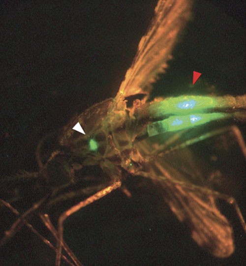
Mosquito seen under a stereozoom microscope with epi-fluorescence and GFP filter. The mosquito was infected with P. berghei GFP-expressing parasites. The salivary glands containing the fluorescent sporozoites are visible in the salivary glands (white arrowhead). Fluorescent parasites are also visible in the midgut (red arrowhead).
Critical Step
As all mosquitoes in a cage are usually not infected, and given that imaging is performed after a single mosquito bite, it is crucial to select mosquitoes with infected salivary glands for the bite session. Select at least 20 mosquitoes with fluorescent salivary glands. Keep these mosquitoes at 21°C and at least 70% humidity, but without sugar solution to starve the mosquitoes and increase their biting behavior the next day.

Preparing for the imaging session
-
4
Prepare the recipient rodent(s) and the selected mosquitoes. Ideally, imaging is performed using hairless mice to avoid autofluorescence of the hair, but C57Bl/6 and BALB/c mice, as well as Brown–Norway rats, have been used successfully after shaving of the ear pinna.
-
5
Turn on the homeothermic heater blanket, install the desired objective (× 10 or × 25), turn on the imaging system and verify that all electronic devices of the imaging system are working properly (lasers on, fan working, motorized stage moving, mercury arc lamp on, software running).
-
6
In the microscope software, open the windows necessary for image acquisition. For tracking sporozoite movement, it is important to privilege rapid acquisition using a large z-slice (approximately 10 μm). For studying sporozoite–host cell interaction, it is important to privilege small z-slice intervals, with or without time. To reduce enormous data files, a binning of 2 × 2 allows sufficient information for cell tracking and cell interactions. The binning can be adjusted according to the desired temporal–spatial resolution. The smaller the binning (e.g., 1 × 1), the better the x, y spatial resolution; however, temporal resolution will be worse (longer exposure times needed) and the files will be bigger. In Image Suite, open the following windows: 'Gallery', 'Experiment', 'Image Control', 'Hardware Controller' and 'Sequence Control'. In 'Gallery', open a new experiment. Go to the 'Image Control' window, set the binning to 2 × 2, increase the gain to the maximum (255) and click on 'full chip' button. Go to the 'Hardware Control' window, 'Dichroic' panel, click on the '488/568/647' button. In the 'Channel settings' panel, channel 'A' option, select the laser to excite on 488 nm and set it to record. In channel 'B', select the laser to excite on 647 nm and set it to record. Adjust the 'Exposure' time to 500 ms. In the 'Power' panel, adjust the laser for maximum power. In 'Stage Control', set the slice spacing to 10 μm if using a × 25 objective, or to 15 μm if using a × 10 objective. For punctual Z-stacks of cell interactions, the z-slice should be reduced, for example, to 0.5 μm. To achieve an optimal 3D reconstruction, the z-step must be at most equal to the thickness of the optical slice or smaller.
Critical Step
The parameters stated here are only an indication and can vary depending on both the samples and the equipment used.
-
7
Test the laser—In the 'Hardware Controller' window, 'Channel settings' panel, click on the channel 'A' button, and a blue light should be seen; click on the channel 'B' button, and a red light should be seen.
Caution
The laser beam can cause serious eye damage. Note that the energy measured at the end of the objective with the spinning disk confocal laser is one order of magnitude lower than the energy from a laser-scanning confocal and two orders of magnitude lower than the energy from the mercury arc lamp.
-
8
Fix a coverslip with adhesive tape over the hole in the platform (see EQUIPMENT SETUP). Install the platform on the microscope and cover with the thermal blanket.
Obtaining the imaging sample
-
9
Anesthetize the recipient mouse (approximately 20 g) by i.p. injection of approximately 100 μl anesthetic.
-
10
Hold the anesthetized animal gently over the cage containing the infected mosquitoes exposing the periphery of the ear pinna (external face) to the selected mosquitoes. Wait for a mosquito to land on the ear and let the insect bite for 1 min. Note the time of bite by using the time on the computer, so that this will correspond to the times on the image files. For example, double-click on the clock at the bottom right corner of the computer to monitor the time of bite. The UltraVIEW software uses the same clock to save the time in the recorded files.
Critical Step
This step requires patience; it can take from a few minutes to hours. In general, 40% of A. stephensi mosquitoes have found a blood source on which to feed in the minute that follows landing on the prey16. Studies on the sporozoite ejection rate during mosquito salivation5,17 have revealed that mosquitoes harboring thousands of sporozoites in their salivary glands could eject either no or over 1,000 sporozoites during a 10-min-long salivation period, while during the first minute of salivation, a mean of 20 sporozoites is ejected. Overall, although the ear pinna is ideal for imaging because of its accessibility and thinness, other sites can be imaged. Note that bites can provoke a local hematoma or not; in the latter case, the site of bite should be memorized using the pattern of superficial veins and marked using nonfluorescent ink.
-
11
Remove the thermal blanket from the microscope stage, place the animal on the heated platform and accommodate the hematoma/bite site at the center of the coverslip, taped on the hole of the platform. Then, tape the ear pinna as flatly as possible to the coverslip.
-
12
Switch on the mercury arc lamp, turn the light path toward the ocular and search for sporozoites using a GFP/fluorescein isothiocyanate filter. If no sporozoites are seen, repeat Steps 11 and 12.
Critical Step
Avoid lengthy exposure to mercury arc lamp illumination; it can cause excess heating of the sample or cell damage via the generation of oxygen radicals and other forms of photoxicity. Many of the deleterious effects are cumulative, which limits the time in which reliable observations can be made.
-
13
Remove the platform with the animal from the microscope carefully, inject 50 μl fluorescent BSA into the retro-orbital sinus using an insulin syringe to label the blood circulation and, if the animal starts to wake up, inject i.p. 25 μl anesthetic.
-
14
Place the platform back on the microscope stage, cover the animal with the thermal blanket, making sure that the bite site is at the center of the hole and find the sporozoites using the mercury arc lamp (Fig. 2).
Figure 2: Experimental setup for imaging sporozoites in the dermis of the murine ear. 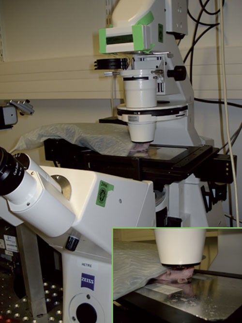
Once the mouse has been bitten, it is placed on the microscope platform so that the site of bite (on the ear) is in the middle of the coverslip over the hole. The ear is then taped into place to avoid any displacement during recording, and the mouse is covered with the homeothermic blanket.
-
15
Prepare for image acquisition by changing the excitation light path from the mercury arc to the laser source and the emission light path from the ocular to the detector. Other changes may be necessary, such as the position of microscope filters.

Acquiring the images
-
16
Activate the 'live image' window and the 488-nm laser to visualize GFP-expressing parasites. Use the microscope controls (focus adjustment knobs and the motorized microscope stage) to focus on the parasites and define the observation field. If there are many parasites in the same field, numerous events will be recorded at the same time. Sporozoites move rapidly, so try to avoid parasites at the edges, as they may move out of the field during the recording. In the 'Experiment' window, click on the 'Live Images' button. Go to the 'Hardware Controller' window in the 'Channel settings' option, and click on the channel A and activate the excitation on 488 nm. The camera image should appear on the monitor.
Focusing
-
17
Focus on the epidermis using the fine adjustment knob and set this as the bottom z-position. In the 'Hardware Controller' window, 'Move' panel, position the z-step controller on 80 μm. The depth of the focal plane is now controlled using the z-step controller in the software.
Setting Z-stacks ('3D snapshots')
-
18
Using the z-step controller (positioned at the bottom, i.e., 80 μm), move the focus toward the top position (i.e., 0 μm). When the first (most superficial) parasite appears, set the Z-stack bottom limit. Using the z-step controller, continue moving toward the 0 μm position. When the deepest parasite is out of focus, set the top limit of the Z-stack.
Critical Step
Usually, a Z-stack of 50 μm is enough to cover the skin volume that contains the parasites delivered during a bite. If the parasite dispersion exceeds 50 μm, using the microscope, focus on the most superficial parasite and reset at that z-position the Z-stack bottom limit (i.e., 80 μm). This step should be done as fast as possible, and is just one among the several ways for adjusting the Z-stack settings.
Setting exposure time and laser power
-
19
Adjust the exposure time and laser power for each laser (i.e., on channel 'A' (488 nm) and 'B' (647 nm)), so that the blood vessels and the parasites are visible.
Critical Step
The time of exposure should be adjusted depending on the number of slices per channel. If the laser power is not already on maximum, it is possible to add power, to keep the exposure time as low as possible. To minimize photobleaching, keep the laser power and total exposure time as low as possible. For time lapse, the ideal conditions are determined by the duration of the experiment with a minimum acquisition time, and a minimum sampling frequency for Z-stacks (i.e., the longest time possible between each Z-stack acquisition, which still allows reasonable temporal resolution of the parasite dynamics; in our case, there is no delay between stacks). In contrast, each Z-stack acquisition should be achieved with the minimal delay between images (ideally continuous acquisition) and the shortest exposure time per image.
Recording movies
-
20
Set the system to record sequences of 10 min. In the 'Sequence Control' window, go to 'Length (sec)' option and set the recording time (we usually record movies of 600 s; see Step 28). Go to 'Grab Options', activate the Z-stack (green) and the time-lapse (red) buttons. Start recording the images by clicking on the gray button with a red circle at the bottom of the 'Sequence Control' window. The 'Experiment' window should show the real-time acquisition.
Critical Step
Looking at the real-time images, check if all parameters (laser, z-step and time of exposure) are properly set. If not, stop the acquisition, correct the parameter and restart recording; i.e., if parasites are not visible, verify that the 'green' channel is being recorded and that the time of exposure is correct.
-
21
When the time of acquisition is completed, check the quality of the recorded images. For example, if parasites remain visible and their movement can be followed, then more sequences can be recorded until the desired length of time has been acquired. In the 'Sequence Control' window, click (gray button with red circle) to record again. Note that when using the Hamamatsu camera (full chip), each image (binning 2 × 2) has 672 × 512 pixels (approximately 340 kb). When recording 600 s-long movies, recording 5 z-slices in both the green and far-red channels with an exposure time of 400 ms per time-point, the computer generates 1,500 pictures to 500 Mb per film.
Critical Step
If necessary, more anesthetic (25 μl) can be injected during recording, but do not move the animal.
Exporting the images
-
22
Export the images as .tif files using the UltraVIEW software. Alternatively, use the Perkin-Elmer 4D-images series converter plugin, written to run in ImageJ, which is freely available at http://www.embl-heidelberg.de/eamnet/html/pe_plugin.html (Marchand, M. and Shorte, S.L., PFID, Institut Pasteur).
Pause point
Once the images have been saved, they can be analyzed immediately or at a later point.
Processing the images: ImageJ and plugins
-
23
Open exported images: in 'File > Import > Image Sequence', select the folder that contains the .tif files exported using the UltraVIEW software. In 'Sequence option > File name contains', type the file name (e.g., '488 nm Z0'). The software will open all files containing this name or all the time points of Z-stack 0 acquired on the 488-nm channel.
Visualizing the position of sporozoites in the Z-stack over time
-
24
The output of imaging is often presented as movie clips made by projecting the z information into a single image by using a method called maximum-intensity projection. This process removes information on where the cells actually lie in the z-dimension, which may result in the impression that two cells come into contact when they actually pass over each other. One method to provide more z-dimension information for the viewer is to change the color of the target dynamically, based on its z-position within the image volume. For instance, the z-slice from 0 to 10 μm in blue, the z-slice from 11 to 20 μm in green and so forth.
Visualizing sporozoite movement over time: merging Z-stacks over time
-
25
To merge three time sets of Z-stacks (Z0, Z1 and Z2), as shown in Figure 3 (see panel b), open each TZ-plane (time points of a given z-plane) as one stack (time points of Z0488 nm = stack0, time points of Z1488 nm = stack1 and time points of Z2488 nm = stack2). In 'Process > Image Calculator', select the stack0 as 'Image1', the stack1 as 'Image2' and the operation as 'Max' (maximum-intensity projection). Click on 'Create New Window' and on the OK button. The resulting stack (stack3) corresponds to the maximum-intensity projections of stack0 and stack1. Repeat this step, now using stack3 as 'Image1' and stack2 as 'Image2'. The resulting stack (stack4) is the maximum-intensity projection of Z0, Z1 and Z2 over time points.
Figure 3: Example of a parasite invading a lymphatic vessel (see Supplementary Video 3). 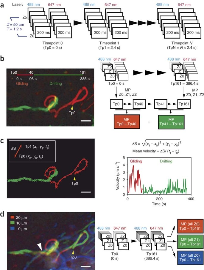
(a) Experimental design. Each time point (Tp) comprises six z-slices recorded sequentially using the laser excitation at 488 nm and six z-slices using the excitation at 647 nm. The exposure time of a single z-slice is 200 ms, totaling 1.2 s per laser channel and 2.4 s per Tp. The z-step is 10 μm using a ×25 immersion objective and binning 4 × 4. (b) Temporal color code. The picture shows the changing of a continuous movement (gliding in red) to a discontinuous passive drifting (lymph drainage in green). The picture is composed by maximum-intensity projections (MIPs) of three Z-stacks (Z-projections) and time points (T-projections), using images acquired on the 488-nm channel. The first step is a Z-projection of three Z-stacks (MIP of Z0, Z1 and Z2; volume of 20 μm) for each time point. These Z-projections between the time points 0 and 40 are again maximum projected (T-projection0–40). After these two steps, the resulting projection represents the movement of the parasite in a flat volume of 20 μm for 96 s (T-projection0–40 of Z-projectionZ0,Z1,Z2). The same is performed with the merged Z-stacks between the time points 41 and 161 (T-projection41–161 of Z-projectionZ0,Z1,Z2). The MIP that corresponds to the gliding movement of the parasite in a volume of 20 μm (T-projection0–40 of Z-projectionZ0,Z1,Z2) was pseudo-colored in red, and the MIP of the lymph drainage (T-projection41–161 of Z-projectionZ0,Z1,Z2) was pseudo-colored in green. Scale bar = 15 μm. (c) Tracking the parasite. The sequence containing the time points of the Z-projectionZ0, Z1,Z2 was thresholded in ImageJ, and the position of each parasite was tracked using the 'multitracker' plugin. The (x, y) position of the selected parasite was plotted for each time point using Microsoft Excel. The velocity is an approximate value of the average velocity between two time points and is calculated by dividing the parasite displacement (ΔS) by the time between two time points (ΔT = 2.4 s). Note the decrease in the velocity when the parasite changes from continuous gliding to passive drifting. (d) Color code of the z-planes. The picture shows that the trajectory of the passively drifting parasite does not coincide with the trajectory of the blood vessels. Each z-plane, acquired using the 488- and 647-nm channels (GFP/parasite and BSA-647/blood, respectively), was projected (MIP) over time and pseudo-colored. T-projection0–16 1 of Z0488 and 647 nm was pseudo-colored in blue and represents the parasite and the blood circulation at 0 μm. T-projection0–161 of Z1488 and 647 nm was pseudo-colored in green and represents the depth of 10 μm. T-projection0–1 61 of Z2488 and 647 nm was pseudo-colored in red and represents the depth of 20 μm. Note the change in color when the parasite switches from continuous gliding to passive drifting, and when the parasite crosses the vessel (white arrowhead).
-
26
To project the time points of stack4, go to 'Images > Stacks > Z-projection' and choose first and last time-points desired for the projection by typing the respective slice number in the options 'start' and 'stop'. Choose the way the slices between 'start' and 'stop' are projected.

Tracking parasites
-
27
Adjust the threshold of the merged Z-stack in 'Image > Adjust > Threshold'. Ideally, the thresholded parasite should appear as a continuous object in all slices tracked. One example is given in Supplementary Videos 1 and 2. Track the thresholded parasites by running the plugin MultiTracker in 'Plugins > Stacks > MultiTracker'. The software will generate a 'Results' table with the (x, y) positions of all tracked objects.
-
28
Export the 'Results' table to a Microsoft Excel sheet and plot the (x, y) trajectory to confirm the parasite track, as shown in Figures 3b and 4 (see panel b). If it is correct, calculate the distance in pixels, as shown in Figure 3c. Also see Supplementary Video 3. Convert the distance to micrometers, and divide by the time between two time points. The result is an average velocity of the thresholded parasite between two sequential images. Note that this velocity is an approximate value since the three Z-stacks are merged.
Figure 4: Example of a parasite invading and gliding inside a blood vessel (see Supplementary Video 4). 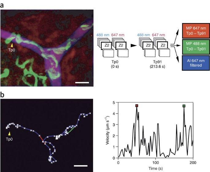
(a) Channel color code. The picture shows a parasite invading a blood vessel. The parasite (green), after invading the vessel (red and blue), glides inside the vessel and is sometimes carried by the blood flow. The image is an RGB image composition of a maximum-inten sity T-projection0–91 of one Z-stack (Z2488 nm), which represents the parasite movement (in green); a maximum intensity T-projection0–91 of one Z-stack (Z26 47 nm), which represents the blood movement during the time point 0–91 (in red) and an average intensity T-projection of ten selected images where the BSA-647 filled the vessel, representing the space occupied by the blood flow or the interior of the blood vessel (in blue). (b) Tracking the parasite. The graphs show the trajectory (left) and velocity (right) of the parasite invading the blood vessel. The intervals when the parasite is moving at high-speed 'jumps', concomitantly with the blood flow, are shown as red/green lines in the trajectorygraph (left) and as red/green squares in the velocity graph (right), confirming the parasite location inside the vessel. Tp0 (time point 0) represents the beginning of the movie. Scale bars = 15 μm.

Visualizing parasites and the blood circulation: pseudo-coloring of stacks
Troubleshooting
Troubleshooting advice can be found in Table 1.
Timing
Step 1, infecting and rearing mosquitoes: 18–22 d
Steps 2–3, selecting infected mosquitoes: 30 min
Steps 4–8, preparation of microscope system and anesthesia of rodent: approximately 30 min
Steps 9–12, bite session: from minutes to hours
Steps 13–19, blood flow labeling and microscope settings: a few minutes
Steps 20, 21: time of recording: approximately 1 h
Steps 22–29: exportation and analysis of images: largely depends on which analyses are to be done. However, the analysis steps can be done at a later time.
Anticipated results
This protocol, which is based on the technology of spinning-disk confocal microscopy that allows for high-speed acquisition of images in a living animal without leading to tissue damage, is useful to image in 4D the behavior of fluorescent Plasmodium sporozoites in the dermis of rodents. Several crucial steps during the infectious process can now be imaged in vivo in quantitative terms, including their motility and interactions with host cells in the dermis, and their passage into the blood or the lymphatic circulation. Examples of images acquired using this protocol are shown in Figures 3 and 4. Figure 3 shows a parasite invading a lymphatic vessel (see Supplementary Video 3). The invasion event is characterized by the switching of a continuous gliding movement (red projection) to a passive drifting (green projection) (Fig. 3a). Figure 3b indicates the decrease of parasite velocity over time. Figure 3c shows the noncoincidence of the path of the passively drifting parasite with the trajectory of the blood. Figure 4 shows a parasite invading a blood vessel and gliding inside the vessel. The colored lines and squares in Figure 4b represent the blood flow carrying the parasite inside the vessel (see Supplementary Video 4).
The future applications of this protocol are numerous. First, analyses using the collection of mutant parasite strains available will improve our understanding of key molecular components necessary for parasite invasion and development. Second, the use of knockout mouse strains will aid in the identification of host components involved in the fate of the parasite. For example, the study of the behavior of parasites in the dermis could be tackled using mice strains affected for extracellular matrix components or endothelial cell junction molecules. In addition, this methodology will be suitable for the study of Plasmodium sp. in their natural host (P. berghei—Grammomys surdaster) or P. falciparum in humanized mice.
Note: Supplementary information is available via the HTML version of this article.
References
Boyd, M.F. & Kitchen, S.F. The demonstration of sporozoites in human tissues. Am. J. Trop. Med. Hyg. 19, 27–31 (1939).
Ponnudurai, T., Lensen, A.H., van Gemert, G.J., Bolmer, M.G. & Meuwissen, J.H. Feeding behaviour and sporozoite ejection by infected Anopheles stephensi . Trans. Roy. Soc. Trop. Med. Hyg. 85, 175–180 (1991).
Sidjanski, S. & Vanderberg, J.P. Delayed migration of Plasmodium sporozoites from the mosquito bite site to the blood. Am. J. Trop. Med. Hyg. 57, 426–429 (1997).
Matsuoka, H., Yoshida, S., Hirai, M. & Ishii, A. A rodent malaria, Plasmodium berghei, is experimentally transmitted to mice by merely probing of infective mosquito, Anopheles stephensi . Parasitol. Int. 51, 17–23 (2002).
Frischknecht, F. et al. Imaging movement of malaria parasites during transmission by Anopheles mosquitoes. Cell. Microbiol. 6, 687–694 (2004).
Natarajan, R. et al. Fluorescent Plasmodium berghei sporozoites and pre-erythrocytic stages: a new tool to study mosquito and mammalian host interactions with malaria parasites. Cell. Microbiol. 3, 371–379 (2001).
Franke-Fayard, B. et al. A Plasmodium berghei reference line that constitutively expresses GFP at a high level throughout the complete life cycle. Mol. Biochem. Parasitol. 137, 23–33 (2004).
Tarun, A.S. et al. Quantitative isolation and in vivo imaging of malaria parasite liver stages. Int. J. Parasitol. 36, 1283–1293 (2006).
Frevert, U. et al. Intravital observation of Plasmodium berghei sporozoite infection of the liver. PloS Biol. 6, e192 (2005).
Vanderberg, J.P. & Frevert, U. Intravital microscopy demonstrating antibody-mediated immobilisation of Plasmodium berghei sporozoites injected into the skin by mosquitoes. Int. J. Parasitol. 9, 991–996 (2004).
Amino, R. et al. Quantitative imaging of Plasmodium transmission from mosquito to mammal. Nat. Med. 12, 220–224 (2006).
Sturm, A. et al. Manipulation of host hepatocytes by the malaria parasite for delivery into liver sinusoids. Science 313, 1287–1290 (2006).
Nakano, A. Spinning-disk confocal microscopy. A cutting-edge tool for imaging of membrane traffic. Cell Struct. Funct. 27, 349–355 (2002).
Sinden, R.E. et al. Maintenance of the Plasmodium berghei life cycle. Methods Mol. Med. 72, 25–40 (2002).
Fay, F.S., Carrington, W. & Fogarty, K.E. Three-dimensional molecular distribution in single cells analysed using the digital imaging microscope. J. Microsc. 153, 133–149 (1989).
Li, X., Sina, B. & Rossignol, P.A. Probing behaviour and sporozoite delivery by Anopheles stephensi infected with Plasmodium berghei . Med. Vet. Entomol. 6, 57–61 (1992).
Medica, D.L. & Sinnis, P. Quantitative dynamics of Plasmodium yoelii sporozoite transmission by infected anopheline mosquitoes. Infect. Immun. 73, 4363–4369 (2005).
Acknowledgements
We thank G. Milon, B. Martin, F. Frischknecht and P. Brey for experiment-related advice and 'real-time' support; A. Genovesico, C. Zimmer and J.C. Olivo-Marin for helping with tracking analysis; E. Perret, P. Roux, M. Marchand and C. Machu for helping with imaging; C. Bourgouin, I. Thiéry and the other members of the Center for Production and Infection of Anopheles for rearing the mosquitoes and B. Franke-Fayard, A. Waters and C. Janse for providing the PbGFPCON parasite. This work was supported by funds from the Pasteur Institute (Stratagic project 'Grand Programme Horizontal Anopholes'), the Howard Hughes Medical Institute and the European Commission (FP6 BioMalPar Network of Excellence).
Author information
Authors and Affiliations
Corresponding authors
Ethics declarations
Competing interests
The authors declare no competing financial interests.
Supplementary information
Supplementary Video 1
Video showing a parasite invading a lymphatic vessel. Video shows the green channel only. Before tracking parasites, this video must be thresholded, as shown in Supplementary Video 2 (MOV 1173 kb)
Supplementary Video 2
Thresholded video showing a parasite invading a lymphatic vessel (MOV 61 kb)
Supplementary Video 3
Invasion of a lymphatic vessel by a sporozoite (yellow arrowhead). Video corresponds to data analysis shown in Figure 3 (MOV 1138 kb)
Supplementary Video 4
Invasion of a blood vessel by a sporozoite (yellow arrowhead). Video corresponds to data analysis shown in Figure 4 (MOV 835 kb)
Rights and permissions
About this article
Cite this article
Amino, R., Thiberge, S., Blazquez, S. et al. Imaging malaria sporozoites in the dermis of the mammalian host. Nat Protoc 2, 1705–1712 (2007). https://doi.org/10.1038/nprot.2007.120
Published:
Issue Date:
DOI: https://doi.org/10.1038/nprot.2007.120
This article is cited by
-
Plasmodium sporozoite search strategy to locate hotspots of blood vessel invasion
Nature Communications (2023)
-
Single-cell RNA sequencing reveals developmental heterogeneity among Plasmodium berghei sporozoites
Scientific Reports (2021)
-
A mouse ear skin model to study the dynamics of innate immune responses against Staphylococcus aureus biofilms
BMC Microbiology (2020)
-
Quantification of wild-type and radiation attenuated Plasmodium falciparum sporozoite motility in human skin
Scientific Reports (2019)
-
TRSP is dispensable for the Plasmodium pre-erythrocytic phase
Scientific Reports (2018)
Comments
By submitting a comment you agree to abide by our Terms and Community Guidelines. If you find something abusive or that does not comply with our terms or guidelines please flag it as inappropriate.
