
Abstract
Imaging mass spectrometry (IMS) allows the direct investigation of both the identity and the spatial distribution of the molecular content directly in tissue sections, single cells and many other biological surfaces. In this protocol, we present the steps required to retrieve the molecular information from tissue sections using matrix-enhanced (ME) and metal-assisted (MetA) secondary ion mass spectrometry (SIMS) as well as matrix-assisted laser desorption/ionization (MALDI) IMS. These techniques require specific sample preparation steps directed at optimal signal intensity with minimal redistribution or modification of the sample analytes. After careful sample preparation, different IMS methods offer a unique discovery tool in, for example, the investigation of (i) drug transport and uptake, (ii) biological processing steps and (iii) biomarker distributions. To extract the relevant information from the huge datasets produced by IMS, new bioinformatics approaches have been developed. The duration of the protocol is highly dependent on sample size and technique used, but on average takes approximately 5 h.
Introduction
It was believed that sequencing the human genome1,2 would lead to a better understanding of biological processes in diseased and healthy organisms. However, it has become apparent that understanding of biological mechanisms cannot be achieved merely by having complete sequences of genomes. The cellular proteome is highly dynamic, and genetic information alone cannot predict the function of a given protein3,4,5. Furthermore, the number of protein-coding genes is far fewer than the number of actual proteins as a result of alternative splicing and post-translational modifications6,7,8,9. Several diseases are associated with altered (or mis)functioning of proteins caused by altered localization10,11,12, post-translational modifications13,14,15,16, or differing expression levels11,17. Numerous proteomic approaches are being used to elucidate elements of this missing information in many different biological processes. Ultimately, methods to study changes in the cellular proteome should interfere as little as possible with the natural behavior of the molecules of interest. Imaging mass spectrometry (IMS) has recently been recognized as a proteomic tool for in situ spatial analysis of molecules in (diseased) tissue5,18. IMS enables the direct investigation of, for example, the effect of a disease or drug treatment on the tissue microenvironment.
IMS
Matrix-assisted laser desorption/ionization-mass spectrometry (MALDI-MS) depicts the localization of biomolecular components such as proteins and peptides directly from tissue19,20,21,22,23,24. The spatial resolution in conventional microprobe IMS has been limited by the laser spot size and sample preparation issues. In microprobe experiments the tissue surface is scanned at an array of predefined points, and at every point a mass spectrum is acquired. The corresponding molecular image is reconstructed after the analysis. The predefined points correspond to the pixels in the resulting image and their size, assumed square, is dependent on the size of the laser spot. The spatial resolution of MALDI imaging has been increased by developing optical lenses able to focus the laser to submicron dimensions25. However, decreasing the laser spot size decreases the efficiency of MALDI for macromolecules. This is caused by the increased laser fluence needed to reach the MALDI threshold when using smaller laser spots26,27, resulting in increased fragmentation of the macromolecules. This implies there will always be a trade-off between signal intensity and spatial resolution in microprobe IMS. Another novel approach to increasing spatial resolution in MALDI-IMS is oversampling with complete sample ablation, developed by Jurchen et al.28 Here the MALDI matrix is ablated completely, after which the sample stage is moved in increments smaller than the size of the laser beam. Although the resulting images show features smaller than 40 μm in size without the need to focus the laser beam, the study of large areas will be extremely time consuming.
Despite the limitation on obtainable spatial resolution, microprobe MALDI-IMS has proven to be a powerful extension of existing proteomic techniques. Sweedler and co-workers showed in 2000 the ability of MALDI-MS to profile peptides in single cells and organelles29,30. In tissue, the localization of amyloid β peptides in relation to Alzheimer's disease31,32, the decrease of a neuronal calmodulin-binding protein (PEP-19) in relation to Parkinson's disease33 and the accumulation of transthyretin Ser28–Gln146 in the cortex of affected kidneys after drug administration34 have been shown using MALDI-IMS. Distinct protein profiles have been obtained when comparing tumor and non-tumor tissue within a single tissue section35. Another very interesting application of IMS is the tracking of administered drugs. Using IMS it is possible to follow not only the parent molecule but also possible metabolites formed after administration32.
Mass microscope
A new approach to IMS decouples the obtainable spatial resolution from the dimensions of the footprint of the ionization beam using a stigmatic mass spectrometric microscope (Fig. 1)36. Here, the desorbed ions retain their original spatial distribution from the tissue surface during their time-of-flight (ToF) separation and are imaged using a 2D position-sensitive detector. This approach allows for high versatility in choosing the ionization method without influencing the obtainable spatial resolution. When the mass microscope is used in combination with MALDI, the spatial resolution depends solely on the quality of the ion optics and the detector resolution; spatial detail can be obtained from within the laser spot. In this method, the spatial resolution obtained in MALDI-IMS is comparable to that obtained in secondary ion mass spectrometry (SIMS) imaging experiments of tissue sections. Using relatively large laser spots (150 × 200 μm2), which is favorable for MALDI efficiency, delivers an image quality of 500-nm pixel size and 4-μm resolving power in both IR and UV MALDI-IMS36,37.

(a) The triple ion focusing (TRIFT) time-of-flight, (b) the matrix-assisted laser desorption/ionization (MALDI) laser source, (c) the CCD camera and (d) instrument control and data acquisition.
In our mass microscopy approach, the 150 × 200–μm2 homogeneous laser pulse irradiates the sample surface. The desorbed ions pass an immersion lens/transfer lens combination followed by a high-speed blanker and are detected at a micro-channel-plate (MCP)/position-sensitive detector (Fig. 2a). In this manner, a mass-to-charge (m/z) separated series of molecular images is generated, allowing simultaneous recording of a microscope and a microprobe dataset in a single experiment. The position-sensitive detector consists of a charge-coupled device (CCD) camera phosphor screen assembly, where snapshots of the ions reaching the detector are taken. These snapshots are used to construct larger area stigmatic ion images. To construct a whole tissue image, several linescans are taken over the entire tissue section by moving the sample stage at a constant speed (typically 100 μm s−1) using a continuously firing laser. At the end of a single linescan, the sample stage is moved upward by 60–80% of the laser spot size and another linescan is taken, until the entire tissue section has been measured. Using software developed in house, all the single stigmatic ion images are stitched together to form a linescan image. These individual linescan images are then combined to form the total image of the entire tissue section. The overlap of the consecutive laser shots is calculated, and the intensity data of the overlapping areas are averaged in the images. The resulting image reveals a high-resolution picture of the sampled surface.

(a) Schematic representation of the Physical Electronics TRIFT-II mass spectrometer. (b) Single laser shot in a matrix-assisted laser desorption/ionization (MALDI) stigmatic imaging experiment without the high-speed blankers on, showing all ions in the MS spectrum and on the phosphor screen [total-ion-count (TIC) image]. (c) Single laser shot in a MALDI stigmatic imaging experiment with the high-speed blankers on, showing only one selected ion in the MS spectrum and on the phosphor screen [selected-ion-count (SIC) image].
As the speed of the CCD camera is insufficient to record the high spatial resolution images for each analyte distribution reaching the detector within one cycle of the experiment, the stigmatic imaging experiment can be conducted in two modes. First, all the ions are allowed to pass through to the detector, to record stigmatic total-ion-count (TIC) images (Fig. 2b), and, second, the TRIFT high-speed blankers are used to record stigmatic selected-ion-count (SIC) images (Fig. 2c). In the second case, the high-speed blankers are used to remove all ions except the ones passing through an approximately 3-μs time window, which is set manually. In the mass spectrum, a single isolated peak can be seen at the selected m/z position. As only this single species reaches the position-sensitive detector, high spatial resolution mass resolved images can be created.
The spatial resolution obtained using the mass microscope is unprecedented and extends IMS capabilities, complementary to existing fluorescence-based techniques. Nevertheless, fluorescence-based techniques achieve superior resolution and allow experiments to be carried out in vivo. The great benefit of IMS is that the biomolecular content of the sample is measured on the basis of an intrinsic property, molecular mass, thus avoiding the need for a fluorescence label. Avoiding the need for labeling in principle allows the technique to resolve all surface molecules that ionize and omit possible interference of the label with the natural behavior/function of the analyte molecule. Simultaneous determination of protein localization, possible post-translational modifications and expression levels can be achieved in a single experiment. The possibility to search for 'unknowns' qualifies IMS as a discovery tool and comparisons can be made between healthy and diseased tissue without prior assumptions.
SIMS
In SIMS38, the sample surface is bombarded with a high-energy primary ion beam between 5 and 25 keV. Typical primary ions used in SIMS are Ga+, Cs+ and In+, with Ga+ able to provide the smallest probe size (less than 10 nm). Although SIMS does not routinely yield intact protein and peptide signals directly from tissue sections, it does have several advantages compared with MALDI. The most important advantage of SIMS over MALDI is the chemical imaging capabilities, routinely delivering submicron spatial resolution39. Furthermore, the SIMS technique is very sensitive and remarkably versatile as it can analyze almost any kind of solid surface40. The bombardment of these solid surfaces with high-energy primary ions will induce damage over a certain depth in the sample, resulting in changes in the molecular structure of the constituents in this area. To prevent imaging of the induced damage, SIMS imaging experiments are conducted using either a dynamic or a static regime. In the dynamic regime, the entire sample surface is eroded in time and the complete top monolayer is removed. Dynamic SIMS is primarily used in quantitative elemental imaging41,42,43 (not the topic of this protocol). In the static SIMS regime, a much lower primary ion dose is used than in dynamic SIMS, resulting in less than 1% of the top surface atoms and molecules interacting with the primary ion beam, and every primary ion strikes a fresh surface region. Consequently, in static SIMS, significantly less fragmentation of the molecular content occurs, which allows the technique to be used in imaging of small organic components44,45,46. To enhance the ionization yield for large intact molecular ions by SIMS, different kinds of surface modifications (MALDI matrices47,48,49,50,51, silver52 and gold53,54,55,56,57) as well as the use of polyatomic primary ion beams58,59,60,61,62,63 have been suggested. Although these methods have been shown to desorb and ionize peptide and proteins from model samples, in direct tissue analysis they are highly biased toward lipids and steroids. One explanation for this phenomenon is the surface sensitivity of the technique. As with SIMS, only the top few monolayers are sampled, and the technique favors the ionization of compounds with surface propensity such as cholesterol and lipids, which are highly abundant in tissue sections.
In this protocol, surface modifications such as metal-assisted (MetA) and matrix-enhanced (ME) SIMS are described for the ionization of intact biomolecular ions, increasing the applicability of SIMS to genuine biological problems. In MetA-SIMS, a very thin layer (approximately 1 nm) of a metal (e.g., gold) is deposited on the sample surface to assist in the desorption/ionization process40,54,55. One crucial factor in this method seems to be the migration of the analytes on the gold surface. In a recent study, we have shown that SIMS signals for both cholesterol and the lipid phosphatidylcholine (PC) increased when these species were deposited on a thin layer of gold. Increased signals for cholesterol were exclusively obtained when the layer of gold was deposited on top of the cholesterol and PC sample22. The same effect was observed in direct MetA-SIMS tissue analysis22 as well as in a MetA-SIMS study of dyes by Adriaensen et al.56
Using ME-SIMS we have demonstrated the possibility of obtaining peptide signals, from a nervous tissue extract from the pond snail Lymnaea stagnalis, identical to those obtained with MALDI-MS, up to m/z 2,590 (ref. 50). The analysis readily identified five known peptides with ME-SIMS using 2,5-dihydroxybenzoic acid as matrix. In ME-SIMS one is not dependent on the migration of the analyte molecules onto the matrix-covered surface as in MetA-SIMS. The matrix is deposited in a wet environment, and the analyte molecules are extracted from the tissue surface. Nevertheless, the bias for species with surface propensity remains, as during drying these species are pushed to the outside of the forming matrix crystals. Furthermore, sample preparation (described in the protocol) is more stringent because the size of the matrix crystals determines the spatial resolution obtainable.
A very recent innovation in MS, not discussed in the protocol, is desorption electrospray ionization (DESI), first described in 2004 by Takats et al.64 Here, charged droplets and ions of solvent are electrosprayed onto the surface to be analyzed. The impact of the charged particles on the surface produces gaseous ions of surface components. The resulting mass spectra are similar to normal ESI mass spectra in that they show mainly singly or multiply charged molecular ions of the analytes. The unique property of this technique is that the mass spectra can be obtained under ambient conditions, which allows the analysis of samples in their native environment65. The range of samples analyzed using this technique is already extensive, even though it is only two years old, and includes pharmaceuticals66,67, explosives68, dyes69,70 and many other analytes, as well as biological samples such as urine, serum and blood64,65,71. The DESI technique has also been used in tissue imaging72 and could possibly move the field of IMS from in vitro to in vivo systems, imaging live systems (such as cell cultures or animal skin) with mass spectrometry. A possible obstacle in conventional microprobe imaging analysis is the spatial resolution, as the DESI beam is in the order of 0.5–1 mm.
Data analysis
In typical IMS analysis, processing the acquired data is more time consuming than the actual measurement itself. Data analysis can become very complex because of the large amount of data produced. As a result, powerful processing and display tools as well as automated data mining techniques are required73. Among the tools available for microprobe IMS datasets is BioMap31,32 (Rausch, M. & Stoeckli, M. (http://www.maldi-msi.org/)), which supports many more imaging modalities, such as optical and positron-emission tomography. It provides a common visualization and storage platform, which allows functionalities such as overlaying of two individual datasets or displaying of regions of interest.
Multivariate statistical methods, and especially principal component analysis (PCA), are established ways to extract information efficiently from large multidimensional datasets74. Combined with different pre-processing and visualization methods, they form a powerful analytical tool for the analysis of hyperspectral datasets such as the ones obtained in IMS. Using these techniques, chemically relevant spectral features can be extracted from large datasets.
Interpretation of MALDI-IMS data should be done very carefully because mixtures of multiple components (e.g., peptides) can show preferential desorption and/or ionization75,76,77,78. Factors influencing the likelihood of ionization of specific peptides are charged side chains, presence of aromatic amino acids, peptide hydrophobicity, size and the ability to form a stable secondary structure75. Furthermore, there is the so-called ion suppression effect, where dominant peptides in the desorption/ionization process suppress ionization of other peptides present at the surface75,76,77.
Sample preparation
Sample preparation in IMS is directed by observing the analytes of interest within the very complex environment of the tissue section. Choosing the appropriate matrix can enhance the sensitivity toward specific molecular moieties79. In general, in MALDI-TOF experiments, α-cyano-4-hydroxycinnamic acid (HCCA) provides the highest sensitivity in peptide analysis and sinapinic acid in protein analysis, and DHB gives good signal intensity in both mass ranges in a single experiment. Typically, the matrices are dissolved in 50:50 water:acetonitrile or water:ethanol solutions with 0.1% trifluoracetic acid (TFA; v/v). The percentage of organic solvent can be varied according to the hydrophobicity of the analytes of interest. An increase of protein signals from cell lysate or tissue sections by the addition of amphiphilic detergents to the matrix solution or by the use of ionic matrices has been reported80,81 (not the topic of this protocol).
Matrix deposition is probably the most difficult part in the sample preparation procedure. Homogeneous matrix crystals have to be formed on the tissue surface with, depending on the technique used, a confined size and without redistribution of the analyte molecules. In microprobe MALDI-IMS, the restraints on the matrix crystal size are less stringent as the laser spot sizes used are in the range of 100–200 μm. For these experiments, techniques such as the acoustic matrix deposition method developed by Aerni et al.82 can suffice. Here the sample is held face down toward the matrix solution and droplets are ejected toward the sample by focused acoustic waves. On seeded tissue sections, the matrix spots formed are 200–300 μm in size. Successful protein imaging at low resolution could be achieved using this technique33,82.
For high-resolution IMS, however, the size of the matrix crystals is a key factor. To make optimal use of the spatial detail observed using the mass microscope, the crystal sizes should be equal to or smaller than the size of a single pixel. In practice, however, the goal is to achieve sufficient protein or peptide signals from matrix crystals smaller than the size of the tissue features of interest. Furthermore, the matrix application method should be robust and reproducible. These requirements can be met if the matrix arrives at the tissue surface in very small droplets before all solvent has evaporated. Matrix solutions can be sprayed into small droplets using pneumatic nebulization (airbrush)22,79 or electrospray nebulization50,83 (Fig. 3), with the electrospray nebulization method giving smaller and more mono-disperse droplets. Automation of pneumatic nebulization is being developed for reproducibility and high-throughput analysis in our laboratory.

Schematic representation of the electrospray setup.
To optimize matrix crystallization, a washing step has to be performed. The solvent composition can be optimized for the experiment at hand. In most cases, the main concern is to wash away as much salt as possible to optimize matrix crystallization. Recent studies have shown that matrix crystallization and analyte incorporation are hampered by the presence of high concentrations of salt. Furthermore, segregation of the salt molecules from the matrix crystals results in an inhomogeneous sample surface where local variations influence the ionization process.49,84,85 Washing the tissue sections can overcome these problems, but great care has to be taken to prevent diffusion of the analyte molecules and/or washing away of the species of interest. The removal of salt from the tissue sections is typically realized by washing in 70–80% ethanol.22,79 Recently, Lemaire et al.86 showed the usefulness of more rigorous washing for the increase of peptide and protein signals, especially from older or even archived tissue sections. They showed that the treatment of tissue sections with organic solvents such as chloroform, acetone, hexane, toluene or xylene resulted in signal enhancement in MALDI direct tissue profiling. In this approach, the tissue sections are not immersed in washing solvent; rather, the solvent is dispensed on top of the sections using a glass syringe. The organic solvents remove interfering lipids and open up different lipid bilayers, resulting in increased signal intensity but possibly also increased molecular diffusion by removal of the lipid structure. Therefore, when using lipid-extracting solvents as washing agent, one has to be particularly careful to prevent diffusion of the molecules of interest, especially using high spatial resolution techniques.
Protocol
As described above, the sample preparation steps are crucial for the success of IMS experiments. From the dissection and sectioning of the tissue to the actual matrix application, the major concern is preparing MS-compatible tissue samples (i.e., tissue samples giving the required information in a direct MALDI-IMS experiment) while preventing analyte diffusion as much as possible. MS compatibility is a key issue in dissection and cryomicrotome cutting of the tissue sections. Blood sticking to the dissected organ should be limited as much as possible, no polymer-based embedding materials can be used and thickness of the tissue sections is limited. Further handling of the tissue samples aims to attain as high as possible signal intensities with as little as possible redistribution of the analyte molecules. The techniques described here are guidelines to the different approaches to IMS. As an example we show the direct MALDI analysis of a rat brain tissue section in both microscope and microprobe mode.
Materials
Reagents
-
Male Wistar rats (Crl:WU) weighing 350 g (Charles River, Germany)
Caution
Experimental procedures should be in accordance with current animal welfare regulations such as the European directives (86/609/EEC).
-
HCCA (Fluka, cat. no. 70990)
Caution
Irritating to the eyes, the respiratory system and the skin.
-
DHB (Fluka, cat. no. 85707)
Caution
Harmful if swallowed and irritating to the eyes, the respiratory system and the skin.
-
Tissues (see REAGENT SETUP)
-
Trifluoracetic acid (Aldrich, cat. no. T6220)
Caution
Harmful by inhalation and causes severe burns; harmful to aquatic organisms; may cause long-term adverse effects in the aquatic environment.
-
HPLC grade water (Riedel-de Haën, cat. no. 34877)
-
Ethanol (Biosolve, cat. no. 05250501)
Caution
Highly flammable.
-
Matrix solution: 15 mg ml−1 DHB or 10 mg ml−1 HCCA in 50% EtOH/0.1% TFA (electrospray deposition, or ESD); 40 mg ml−1 DHB or 10 mg ml−1 HCCA in 50 % EtOH/0.1% TFA (pressure-driven deposition)
-
Gelatine (De Twee Torens, Delft, The Netherlands)
-
Liquid isopentane
Caution
Isopentane can affect you when inhaled and can irritate the skin, causing a rash or burning feeling on contact; exposure to isopentane can irritate the eyes, nose and throat and can cause headache, nausea, weakness, dizziness, sleepiness, loss of coordination and even loss of consciousness; repeated or prolonged contact with isopentane can cause drying and cracking of the skin; isopentane is a highly flammable liquid and a dangerous fire hazard.
-
Washing solution (1 and 2): ice-cold 70% ethanol
Equipment
-
Dissection microscope allowing low magnification (× 10/ × 40) (CETI, Antwerp, Belgium)
-
Cryomicrotome (Leica CM 3000 cryostat; Leica Microsystems, Nussloch, Germany)
-
Conductive glass slides (25 × 50 × 1.1 mm3 unpolished float glass, SiO2 passivated/indium–tin-oxide (ITO) coated, Rs = 6 ± 2 Ω; Delta Technologies, cat. no. CG-40IN-1115)
-
Sample plate (SS, 100 well, numbers only; Applied Biosystems, cat. no. V503841)
-
Freezer (−80 °C)
-
Optical microscope (Leica DMRX; Leica) equipped with a digital camera (Nikon DXM1200; Nikon)
-
Chromatography sprayer (10 ml; Sigma-Aldrich, cat. no. Z529710)
-
9-mm screw-top vials, 12 × 32 mm2 (Waters, P/N, cat. no.186000272)
-
Digitizer card (Acqiris, Switzerland)
-
Gastight syringe (Hamilton)
-
Translation stage (Thorlabs)
-
Digital micrometer (Mitutoyo)
-
XY movable table (Thorlabs)
-
Syringe pump (KD Scientific)
-
SC7640 sputter coater (Quorum Technologies; Newhaven, East Sussex, UK) equipped with a gold target (SC510-314A), an FT7607 quartz crystal microbalance stage and an FT7690 film thickness monitor
-
TRIFT-II (triple focusing time-of-flight) SIMS (ToF-SIMS) equipped with a 115In+ liquid metal ion gun (Physical Electronics, Eden Prairie, MN)
-
CCD camera (LaVision, Germany)
-
4700 proteomics MALDI TOF/TOF analyzer equipped with a 200-Hz Nd:YAG laser (Applied Biosystems)
Reagent setup
-
Tissue samples Freeze tissue directly in liquid isopentane after dissection, cool on dry ice and store at −80 °C until use. When needed, embed the tissue in compatible embedding material. For very small organs such as the pituitary gland or a mollusk CNS, problems can arise during the cryomicrotome cutting process. Because of the small size of the organs, placement on the sample holder without contact with the support material is unlikely. Furthermore, the cutting of these small organs without embedding material increases the likelihood of damage in the resulting tissue sections, by rumpling or tearing. Embedding in non-polymer-containing solutions such as 10% gelatin or agarose helps to prevent damaging the tissue and assist in cutting. Tissue is embedded in 10% gelatin at 30 °C directly after dissection and frozen at −80 °C. Gelatin embedding allows sectioning down to 5-μm thickness, results in no tissue damage during freezing and is compatible with MS.
Critical
Recent observations by Svensson et al.87 point toward postmortem changes in the proteome of susceptible peptides and proteins within minutes. To prevent these alterations of a sample, Svensson et al.87 use focused microwave irradiation to kill the animals. Since focused microwave irradiation is not available in every laboratory, an alternative way to minimize alterations is snap-freezing of the dissected tissue and defrosting just before sample preparation starts.
Critical
Never embed the tissue in polymer containing cryopreservative solution such as Tissue-Tek O.C.T. Compound (Sakura Finetek USA, Inc., cat. no. 4583). Cryopreservative solutions will smear over the tissue surface during cutting, and in the MS analysis the polymer signals will dominate.
Equipment setup
-
Home-built ESD setup In this setup, a syringe pump (KD Scientific) pumps matrix solution (10–50 μl min−1) from a gastight syringe (Hamilton) through a stainless steel electrospray capillary (OD 220 μm, ID 100 μm) maintained at 3–5 kV (0–6 kV power supply, Heinzinger). The capillary is mounted on an electrically isolated manual translation stage (Thorlabs) in a vertical orientation. The stage is fitted with a digital micrometer (Mitutoyo) for accurate positioning of the needle tip with respect to the grounded sample plate. The sample plate is mounted on an XY movable table (Thorlabs).
-
Mass spectrometer Physical Electronics TRIFT-II mass spectrometer equipped with an MCP/phosphor screen/CCD camera (LaVision) optical detection combination and a MALDI ionization source (described in detail in ref. 36). The instrument is equipped with a DP214 digitizer card with 1-GHz bandwidth and 2 GS s−1 sampling rate (Acqiris) for readout of the MCP signals.
-
Software (i)Both TRIFT systems are operated by WinCadence software (version 3.7.1.5) and controlled by the vacuum watcher (Physical Electronics, Watcher 2.1.2.140). AcqirisLive 2.11 controls the Acqiris settings and data acquisition. LaVision DaVis 6.2.3 controls the CCD camera settings and data acquisition. Mass spectral data analysis is performed with WinCadence 3.7.1.5, MatLab 7.0.4 (PCA), AWE3D 1.5.2.0 and tofToCsv (a tool to convert the entire m/z data file to a comma-separated .csv file). Image data analysis is performed with WinCadence 3.7.1.5, MatLab 7.0.4 (PCA), DataCubeViewer, spatial image composer and tof.bat. All software developed in our laboratory is available to other researchers on request. (ii) The Applied Biosystems 4700 proteomics MALDI TOF/TOF analyzer is operated using the 4000 Series Explorer software. For imaging experiments an extra software package (4000 Series Imaging) is required, which is freely available at http://www.maldi-msi.org. Both mass spectral analysis and image data analysis are performed using the BioMap software, which is freely available at http://www.maldi-msi.org.
Procedure
Preparation of the tissue sections
-
1
Place the dissected tissue on the sample holder in the cryostat. The tissue section can be attached to the sample holder by a very small amount of Tissue-Tek. Great care has to be taken that the Tissue-Tek does not come into contact with the tissue area of interest.
-
2
Cut the tissue section into approximately 10-μm thicknesses using a cryomicrotome at −20 °C. For IMS, 10-μm thickness is optimal; there are enough analyte molecules available for extraction and no problems with isolation.
-
3
Pick up the tissue sections with either microscope glass slides or manufacturer sample plates by thaw mounting (i.e., the tissue sticks to the glass or steel because it thaws slightly upon touching); place them in a closed container (e.g., plastic Petri dishes sealed with parafilm) on dry ice and store at −80 °C until use.
Critical Step
ITO glass slides show best performance in both microprobe and microscope mode imaging because of the preserved conductivity of the sample.
-
4
Take a tissue section in its closed container from the −80 °C storage and allow it to come to room temperature (∼ 20 °C) in a dry box with silica gel canisters before analysis.
Critical Step
When the samples are taken out of the −80 °C freezer, water condenses on them. For this reason samples are packed in Petri dishes closed by parafilm to prevent wetting of the tissue surface. The whole dish is placed in a desiccator until the condensed water has been removed, after which the tissue is taken out of the Petri dish for washing.
-
5
Wash the tissue sections. The washing step is optional depending on the type of analysis.
Critical Step
For SIMS analysis of small molecules such as lipid messengers, steroids or even elemental distributions, the washing step is omitted to prevent diffusion. Also, in the analysis of drug delivery systems, no washing step is used for this same reason. For macromolecular analysis the washing is dependent on the type of analysis, and the washing solution can be altered accordingly. For medium-size peptide analysis (i.e., approximately 1,000–5,000 Da) best results are obtained by washing twice in ice-cold 70% ethanol. Washing is achieved by following these steps: (i) place the glass slide containing the tissue section in the first washing solution by immersing very gently and do not stir or shake. (ii) Leave the slide for 1 min in the first washing solution and than take it out very gently and remove any big drops from the slide. (iii) Place the sample, again as gently as possible, in the second, fresh, washing solution for 1 min. (iv) After the second washing step take out the slide, keep it in horizontal and gently blow a stream of nitrogen over the surface to assist in drying. (v) Place the tissue in the desiccator to let the tissue dry completely; otherwise the tissue may detach from the glass slide and start to ripple.
Critical Step
Careful washing is critical in high spatial resolution imaging. To prevent diffusion of the analyte molecules, place the sample in the washing solution as gently as possible and leave it untouched.
-
6
Use different matrix deposition methods depending on the spatial resolution required. For high spatial resolution IMS, matrix deposition is achieved either by ESD (option A), in SIMS, or pressure-driven spray (option B) in MALDI. The choice of matrix again determines the spatial resolution that can be obtained.
-
A
ESD
-
i
Pump matrix solution, 15 mg ml−1 DHB or 10 mg ml−1 HCCA in 50% EtOH/0.1% TFA, from a gas-tight syringe through a stainless steel electrospray capillary maintained at 3.7 kV for 10 min at a flow rate of 12 μl h−1. The needle-to-sample plate distance is 5.0 mm. No drying or nebulization gas is used.
Critical Step
Key issues in development of a matrix deposition method are optimal incorporation of analyte into the matrix crystals and minimal lateral diffusion. These two requirements can be met if the matrix arrives at the tissue surface in very small droplets before all solvent has evaporated.
-
ii
Check matrix coverage using an optical microscope.
-
iii
Let the tissue sections dry for 30 min.
-
i
-
B
Pressure–driven deposition
-
i
Use a TLC sprayer to spray matrix solution, 10 mg ml−1 HCCA or 40 mg ml−1 DHB in 50% EtOH/0.1% TFA, at a nitrogen pressure of 0.3–0.4 bar. Use several spray cycles to achieve homogeneous matrix coverage and allow the tissue to dry between spray cycles in a horizontal position.
-
ii
Check matrix coverage using an optical microscope.
-
iii
Let the tissue sections dry before gold coating (30 min).
-
i
-
A
Gold coating for MetA-SIMS and stigmatic MALDI-IMS experiments
-
7
For MetA-SIMS coat the tissue sections with 1 nm of gold directly on the tissue, and for MALDI coat the matrix-covered tissue sections with 4 nm of gold. This is done as follows: (i) place the ITO slide with the sample in the Quorum Technologies SC7640 sputter coater. Make sure a gold target is installed. (ii) Press the start sequence button to pump down, flush with argon, further pump down the vacuum chamber and leak in argon until the pressure reaches 0.1 mbar (all done automatically). (iii) Enter the density of the metal used (19.30 g cm−3 for gold) and the desired thickness of the sputtered metal layer. (iv) Put the discharge voltage on 1 kV and press start. (v) Adjust the plasma current to 25 mA for homogeneous coverage.
Critical Step
If the layers are too thick, only gold clusters will be observed.
Imaging mass spectrometry experiments
-
8
Now perform the IMS experiment. IMS experiments described here are ME-SIMS, MetA-SIMS and MALDI experiments. The SIMS experiments are conducted on a Physical Electronics TRIFT-II equipped with a 115In+ liquid metal ion gun. Stigmatic MALDI experiments are performed on a Physical Electronics TRIFT-II equipped with a phosphor screen/CCD camera optical detection combination and a MALDI ionization source. The microprobe MALDI experiments are performed on an Applied Biosystems 4700 proteomics analyzer. The experimental procedures for the ME-SIMS and MetA-SIMS experiments are the same (option A), but different from that for stigmatic MALDI (option B) and microprobe MALDI (option C).
-
A
ME–SIMS and MetA–SIMS
-
i
Optimize setup for image quality. Before conducting SIMS imaging experiments, optimize the setup for image quality, using a copper grid with a 25-μm repeat. In the vacuum watcher, close spectro gate valve (V5). In WinCadance software go to hardware, start the DC beam and raise the gain of the electron multiplier until the copper grid becomes visible on the secondary electron detector (SED).
-
ii
Select lens 1 and wobble. Use the multiple variable aperture, on the side of the instrument, to improve the image quality. When the best result is achieved, stop wobble, select lens 2 and start wobble again. Adjust beam steering (x and y) to improve the image quality when needed. At the optimal image quality, stop wobble, select blanker and start wobble again. This time adjust lens 2 to fix the image and lens 1 to refocus. After the refocusing, the procedure is repeated until a clear fixed and focused image of the copper grid can be seen on the SED.
-
iii
In hardware make sure there is no voltage on the bunching parameter (perform the imaging measurements in unbunched mode for optimal image quality). Before the start of the experiment select, under “acquisition/setup/advanced settings,” “save as raw file” to post-process the raw data after the measurement is completed.
-
iv
The experiment. Perform the ME- or MetA-SIMS experiment in such a way that the analysis is conducted in the static SIMS regime. This can be achieved with a primary ion beam current of approximately 450 pA, a primary pulse length of 30 ns, a spot diameter of 500 nm and a primary ion energy of 15 kV. At 3 min per experiment this results in a primary ion dose of 4.9 × 10¹¹ ions cm−2.
-
v
For each chemical image, raster the primary beam over a 150 × 150 μm2 sample area, divided into 256 × 256 square pixels (larger or smaller areas can also be chosen). To image a significantly larger surface, such as a whole tissue section, analyze multiple 150 × 150 μm2 areas by stepping the sample stage in a mosaic pattern. To compensate for small deviations on the sample stage positioning take a 10-μm overlap with the previous acquired sample (the sample stage is moved by 140 μm).
-
vi
Analyze the data as described in Step 9.
-
i
-
B
Stigmatic MALDI–IMS
-
i
Optimize setup for image quality. Before conducting stigmatic MALDI imaging experiments, optimize the setup for image quality using a fine-mesh TEM grid (19-μm squares, 25-μm pitch) overlaid on analyte-doped matrix crystals. Optimize sample potential, immersion lens and transfer lens voltages to obtain a focused image of the grid structure on the phosphor screen.
-
ii
The experiment. Set sample stage velocity to 0.1 mm s−1 and the laser repetition rate at 10 Hz.
-
iii
Calculate the number of laser shots needed to complete one linescan over the tissue section and use this number as value for the number of images saved from the phosphor screen and mass spectra acquired.
-
iv
After one linescan move the sample stage up by 60–80% of the laser spot size and acquire another linescan. Repeat this step until the entire tissue section has been measured.
-
v
Analyze the data as described in Step 10.
-
i
-
C
Microprobe MALDI–IMS
-
i
Load the ABI sample plate into the 4700 proteomics analyzer and determine the tissue section boundaries.
-
ii
Take a test spectrum outside the tissue section to determine the acquisition method.
Critical Step
The maximum number of data points per spectrum must always be lower than 32,767. Increase the bin size or reduce the mass range to meet this criterion.
-
iii
Select “Manual Acquisition” with one spectrum, define up to 255 laser shots (100 laser shots in our case) and load the 4700 imaging tool (freely available at http://www.maldi-msi.org).
-
iv
Set the coordinates of the tissue section boundaries and give the raster size; the number of pixels on the XY scale is calculated using the dimensions button.
Critical Step
Increasing the number of pixels increases the level of detail in the imaged section. However, the size of the laser beam has to be taken into account to avoid multiple sampling of the same position.
-
v
Give a file name and start the acquisition.
-
vi
Analyze the data as described in Steps 11 and 12.
-
i
-
A
Data analysis
-
9
ME-SIMS and MetA-SIMS (right after Step 8A(iv)). In the WinCadence software, save each individual experiment as a raw file to allow post-processing of the data. In “spectra” choose specific m/z ranges and select “image” for each range. Now in “acquisition/set-up/advanced settings” select “acquire from raw file”; under the tab “image” the selected distributions can be seen. For large tissue sections multiple imaging experiments are performed to cover the entire area. Viewing the tissue section in one image, made up out of the multiple experiments, can be accomplished by combining (stitching) the individual images. Two approaches to image stitching are available. First, 150-μm2 images can be stitched together manually in image handling software such as Adobe Photoshop. Second, PCA-based methods are used to generate feature-based registration of the imaging data cubes for the visualization of the imaging data88.
-
10
Stigmatic MALDI-IMS (right after Step 8B(iv)). As two datasets are being recorded simultaneously, process the data separately and combine them afterwards. The mass spectra can be analyzed as single-shot spectra, as combined spectra per linescan or as combined spectra of the whole measurement. Microprobe images can be created with high detail per single mass or at low detail for every mass, and PCA routines89 can be used to find correlations between distributions of m/z species. The stigmatic ion images can be stitched together showing either the TIC image of the entire tissue section or a high-resolution selected ion distribution.
-
A
Mass spectral analysis
-
i
Acquire the MALDI mass spectral data using an Acqiris digitizer, which results in a single .data file for every laser shot.
-
ii
Visualize the mass spectral data as single-shot spectra per linescan in the 3D tool of AWE software90. A contour plot shows the m/z data on the x-axis and the selected ion current on the y-axis. The intensity data are presented in the z-direction as a heat plot, allowing 3D visualization of the data. Using awe3D, specific m/z species can be visualized per linescan without losing low abundant signals in averaging logarithms.
-
iii
Use Matlab routines to add mass spectral data of a single linescan. These routines help in fast evaluation of the m/z species observed.
-
iv
Use a Java routine (tofToCsv) to convert the entire mass spectral dataset into a comma-separated file, which can be visualized (e.g., in Origin).
-
i
-
B
Stigmatic image stitching
-
i
Stitch the stigmatic ion images together to form a linescan. Then combine these individual linescans to form the image of the entire tissue section (Fig. 4a). The in-house-developed software calculates the overlap of the consecutive laser shots and adds the intensity data for the overlapping areas in the images.
Figure 4: Example of images obtained with microscope matrix-assisted laser desorption/ionization imaging mass spectrometry. 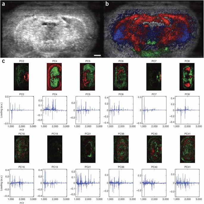
(a) High-resolution microscope mode total-ion-count (TIC) image of a rat brain tissue section. (b) The same microscope mode TIC image with overlaid microprobe m/z data (m/z 1,085 (vasopressin) in green, m/z 2,030 in red and m/z 1,431 in blue). (c) Correlation between different m/z species found in the microprobe dataset of the rat brain tissue section by PCA. Scale bar = 1 mm.
-
i
-
C
Microprobe images
-
i
Create detailed images using the Java-based software, which calculates intensity data for manually selected masses per laser shot position. This low-resolution microprobe dataset is visualized, taking into account the sample stage velocity, laser repetition rate and distance between linescans and can be overlaid with the stigmatic ion images (Fig. 4b). Image processing is done in imaging software such as Adobe Photoshop. Note: Software programs such as Photoshop use automatic smoothing tools when rescaling or resampling images.
-
ii
Visualize the low-resolution images of the entire microprobe dataset using DataCubeViewer. Here, one can scroll through the entire mass spectral dataset showing the 2D localization at every m/z value with the intensity data in the z-direction (comparable to the BioMap software).
-
i
-
D
PCA
-
i
For the PCA, read the Acqiris ADC signals using MatLab (version 7.0.4, R14, SP2). The maximum size of the dataset depends on the available memory. As the IMS datasets consist of relatively large areas with zero counts, the data are stored in a Harwell–Boeing format, which omits the storage of zero counts. To further reduce the data size, binning is performed in the spectral domain. PCA is used to describe the original data using a preselected number of principal components. These components are calculated to describe a percentage in variation (the variance) of the original spectral data. The components are calculated in descending order of variance. In this manner different correlated molecular components can be imaged together, rather than generating images of each individual peak in the dataset. As shown in Figure 4c, a single principal component contains both a positive and negative spatial correlation (on the positive and negative scale in the graph and in red and green in the image). Many different types of spectral correlations can be found; for example, the negative correlation in principal component 2, in Figure 4c, consists mainly of different pseudomolecular ions of the neuropeptide vasopressin. This technique can assist in finding biological processing steps in specialized regions in the tissue.
-
i
-
A
-
11
Microprobe MALDI-IMS (right after Step 8C(iv)). For the data analysis of the microprobe MALDI-IMS experiment we use the BioMap 3.7.4 software, which is freely available at http://www.maldi-msi.org. In our example we obtained the IMS dataset on an Applied Biosystems 4700 proteomics analyzer, which creates a BioMap-compatible .img file. However, datasets obtained with the Bruker Reflex IV or the Ultraflex II are also compatible with the BioMap software after an additional conversion routine (available free of charge; details are described by Clerens et al.91). Load the IMS dataset into BioMap by choosing the .img file in “file/import/MSI.”
Critical Step
BioMap loads the entire dataset into the computer's virtual memory, and thus sufficient memory is needed (for medium-sized datasets, 2 GB).
-
12
Once the dataset has been loaded into BioMap, use the multiple visualization and data handling routines available. As the possibilities are too extensive to discuss in this protocol, only some of the basic steps to visualizing the data are discussed. Example images obtained from a microprobe IMS experiment and processed with the BioMap software are shown in Figure 5. (i) The summed spectra of the imaging experiment can be visualized in the plot tool (“analysis/plot/global/scan”). (ii) Contrast of the selected m/z images can be adjusted by adjusting the minimum and maximum intensity values on the slide-bars in left-side toolbar. The data are automatically shown as interpolated (smoothed) images. For the real (pixelated) image, one has to choose “voxel” instead of “interpolate” in the “display methods” of the image properties window (right mouse click on image), as shown in Figure 5c. (iii) Different m/z images can be selected either by scrolling through the mass spectrum in the plot tool or by adjusting the value of the data points in the left-side toolbar. (iv) The color of the images shown can be changed in the left-side toolbar by choosing the “Set color table” button.
Figure 5: Example of images obtained with microprobe matrix-assisted laser desorption/ionization imaging mass spectrometry on an Applied Biosystems 4700 proteomics analyzer and processed with BioMap software. 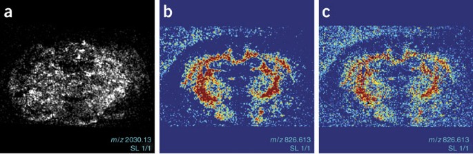
(a) Distribution of a selected mass (m/z 2,030) in gray scale and (b) of a selected mass (m/z 826.6) in color scale (split blue–red). (c) Same image as in panel b but now without interpolation.


Troubleshooting
Step 6B(i)
The pressure on the sprayer is adjusted according to matrix solution used. For higher concentration solutions, a higher pressure is needed. In addition, after several spray cycles sometimes a little higher pressure is needed owing to small deposits of the matrix in the sprayer's tubes. The average pressure used is 0.3–0.4 bar.
As the TLC sprayer's solution reservoir is relatively large compared with the amount of matrix solution needed to cover a single tissue section, use a smaller container (9-mm screw-top vials, 12 × 32 mm2 from Waters) filled with the matrix solution and placed inside the TLC container.
Timing
Step 4, defrosting and drying of tissue sections: 30 min
Step 5, washing and drying of the tissue sections: 10 min
Step 6, electrospray matrix deposition: 10 min (highly dependent on the size of the tissue section); pressure driven deposition: 30 min
Step 7, gold deposition: 6 min (approximately 1.5 min per nm)
Step 8, highly dependent on the size of the tissue section: ME-SIMS analysis: 3 min per 150 μm2 area of the tissue section. Stigmatic MALDI-IMS: for a rat brain tissue section (approximately 1.5 × 0.9 mm2) take a linescan of 1,550 shots, which corresponds to 155 s. With a 120-μm stepsize between linescans, 70 linescans are needed to complete the tissue section. This results in 3 h pure measuring time. Together with resetting all the parameters at the beginning of the measurement of each linescan, a whole tissue section takes approximately 4 h to measure. Microprobe MALDI-IMS of a single rat brain tissue: approximately 4 h to measure, depending on number of pixels and number of laser shots per pixel.
Step 9, the construction of a single image: approximately 0.5 min; stitching of multiple images: 1 h (using PCA software). The stitching of multiple images by hand is more time consuming and can take several hours, depending on the sample size. Using PCA software this can be done much more quickly, depending on data size, processor speed and available memory, typically within 1 h.
Step 10, data analysis for MALDI-IMS using DataCubeViewer or PCA-based software, where both images and spectral information are processed at once, is relatively rapid. The limiting factor is the size of the dataset in combination with available processing power and memory. Loading and processing of the dataset typically takes 1 h, after which all information is readily available. Information extracted using DataCubeViewer and PCA can be analyzed in detail with the software tools described above.
Step 11, data analysis for microprobe MALDI-IMS using the BioMap software, is relatively fast. The loading of the dataset takes typically not more than 10 min, after which the data are readily available for investigation.
Note: The timing of a single IMS experiment is difficult to indicate as this is very much dependent on the size of the sample to be analyzed. Furthermore, the time needed for data analysis depends to a great extent on the questions asked. For example, if IMS is used to find information on a known species in the sample, the answer can be found relatively quickly after data processing. If, on the other hand, one is using the IMS technique as a discovery tool and, for example, wants to discriminate between (drug-)treated and untreated or diseased and healthy tissue, the data mining and comparison will take considerably longer.
Anticipated results
These protocols for IMS allow the mapping of molecular distributions directly in tissue sections. The different approaches to SIMS are able to deliver images of distributions of small organic compounds such as lipids, steroids and drugs within single cells. Figure 4 shows a typical set of images obtained using MALDI-IMS. In Figure 4a, a TIC image of the rat brain tissue section shows the high spatial resolution imaging capabilities of the mass microscope. Figure 4b shows that, in the same experiment, recorded m/z data can be used to show the distribution of both known and unknown species observed in the mass spectrum. In Figure 4c, PCA and varimax analysis are used to show the localization of correlated molecular species within the features of the tissue section. The correlation found between the different molecular species can assist in the search for biological processing steps in specific areas of the tissue at cellular-length-scale spatial resolution.
References
Venter, J.C. et al. The sequence of the human genome. Science 291, 1304–1351 (2001).
Lander, E.S. et al. Initial sequencing and analysis of the human genome. Nature 409, 860–921 (2001).
Pandey, A. & Mann, M. Proteomics to study genes and genomes. Nature 405, 837–846 (2000).
Figeys, D. Proteomics approaches in drug discovery. Anal. Chem. 74, 412A–419A (2002).
Hanash, S. Disease proteomics. Nature 422, 226–232 (2003).
Grabowski, P.J. & Black, D.L. Alternative RNA splicing in the nervous system. Prog. Neurobiol. 65, 289–308 (2001).
Chung, J.J., Shikano, S., Hanyu, Y. & Li, M. Functional diversity of protein C-termini: more than zipcoding? Trends Cell Biol 12, 146–150 (2002).
Stamm, S. et al. Function of alternative splicing. Gene 344, 1–20 (2005).
Aebersold, R. Constellations in a cellular universe. Nature 422, 115–116 (2003).
Zaccai, M. & Lipshitz, H.D. Role of Adducin-like (hu-li tai shao) mRNA and protein localization in regulating cytoskeletal structure and function during Drosophila oogenesis and early embryogenesis. Dev. Genet. 19, 249–257 (1996).
Phizicky, E., Bastiaens, P.I., Zhu, H., Snyder, M. & Fields, S. Protein analysis on a proteomic scale. Nature 422, 208–215 (2003).
Calero, M. et al. Dual prenylation is required for Rab protein localization and function. Mol. Biol. Cell 14, 1852–1867 (2003).
Wang, J.Z., Grundke-Iqbal, I. & Iqbal, K. Glycosylation of microtubule-associated protein tau: an abnormal posttranslational modification in Alzheimer's disease. Nat. Med. 2, 871–875 (1996).
Dierks, T. et al. Multiple sulfatase deficiency is caused by mutations in the gene encoding the human C(alpha)-formylglycine generating enzyme. Cell 113, 435–444 (2003).
Raina, A.K. et al. Acetylation: A novel posttranslational modification in Alzheimer disease. J. Neuropath. Exp. Neur. 62, 551–551 (2003).
Guo, L., Munzberg, H., Stuart, R.C., Nillni, E.A. & Bjorbaek, C. N-acetylation of hypothalamic alpha-melanocyte-stimulating hormone and regulation by leptin. Proc. Natl. Acad. Sci. USA 101, 11797–11802 (2004).
Hoozemans, J.J.M. et al. The unfolded protein response affects neuronal cell cycle protein expression: implications for Alzheimer's disease pathogenesis. Exp. Gerontol. 41, 380–386 (2006).
Aebersold, R. & Mann, M. Mass spectrometry-based proteomics. Nature 422, 198–207 (2003).
Stoeckli, M., Chaurand, P., Hallahan, D.E. & Caprioli, R.M. Imaging mass spectrometry: a new technology for the analysis of protein expression in mammalian tissues. Nat. Med. 7, 493–496 (2001).
Pierson, J., Svenningsson, P., Caprioli, R.M. & Andren, P.E. Increased levels of ubiquitin in the 6-OHDA-lesioned striatum of rats. J. Proteome Res. 4, 223–226 (2005).
Pierson, J. et al. Molecular profiling of experimental Parkinson's disease: Direct analysis of peptides and proteins on brain tissue sections by MALDI mass spectrometry. J. Proteome Res. 3, 289–295 (2004).
Altelaar, A.F.M. et al. Gold-enhanced biomolecular surface imaging of cells and tissue by SIMS and MALDI mass spectrometry. Anal. Chem. 78, 734–742 (2006).
Skold, K. et al. Decreased striatal levels of PEP-19 following MPTP lesion in the mouse. J. Proteome Res. 5, 262–269 (2006).
Altelaar, A.F.M. et al. High-resolution MALDI imaging mass spectrometry allows localization of peptide distributions at cellular length scales in pituitary tissue sections. Int. J. Mass Spectrom. 260, 203–211 (2007).
Spengler, B. & Hubert, M. Scanning microprobe matrix-assisted laser desorption ionization (SMALDI) mass spectrometry: instrumentation for sub-micrometer resolved LDI and MALDI surface analysis. J. Am. Soc. Mass Spectrom. 13, 735–748 (2002).
Dreisewerd, K., Schurenberg, M., Karas, M. & Hillenkamp, F. Influence of the laser intensity and spot size on the desorption of molecules and ions in matrix-assisted laser-desorption ionization with a uniform beam profile. Int. J. Mass Spectrom. 141, 127–148 (1995).
Knochenmuss, R. A quantitative model of ultraviolet matrix-assisted laser desorption/ionization. J. Mass Spectrom. 37, 867–877 (2002).
Jurchen, J.C., Rubakhin, S.S. & Sweedler, J.V. MALDI-MS imaging of features smaller than the size of the laser beam. J. Am. Soc. Mass Spectrom. 16, 1654–1659 (2005).
Li, L., Garden, R.W. & Sweedler, J.V. Single-cell MALDI: a new tool for direct peptide profiling. Trends Biotechnol. 18, 151–160 (2000).
Rubakhin, S.S., Garden, R.W., Fuller, R.R. & Sweedler, J.V. Measuring the peptides in individual organelles with mass spectrometry. Nat. Biotechnol. 18, 172–175 (2000).
Stoeckli, M., Staab, D., Staufenbiel, M., Wiederhold, K.H. & Signor, L. Molecular imaging of amyloid beta peptides in mouse brain sections using mass spectrometry. Anal. Biochem. 311, 33–39 (2002).
Rohner, T.C., Staab, D. & Stoeckli, M. MALDI mass spectrometric imaging of biological tissue sections. Mech. Ageing Dev. 126, 177–185 (2005).
Skold, K. et al. Decreased striatal levels of PEP-19 following MPTP lesion in the mouse. J. Proteome Res. 5, 262–269 (2006).
Meistermann, H. et al. Biomarker discovery by imaging mass spectrometry: transthyretin is a biomarker for gentamicin-induced nephrotoxicity in rat. Mol. Cell. Proteomics 5, 1876–1886 (2006).
Chaurand, P., Schwartz, S.A. & Capriolo, R.M. Profiling and imaging proteins in tissue sections by MS. Anal. Chem. 76, 86A–93A (2004).
Luxembourg, S.L., Mize, T.H., McDonnell, L.A. & Heeren, R.M. High-spatial resolution mass spectrometric imaging of peptide and protein distributions on a surface. Anal. Chem. 76, 5339–5344 (2004).
Luxembourg, S.L., McDonnell, L.A., Mize, T.H. & Heeren, R.M.A. Infrared mass spectrometric imaging below the diffraction limit. J. Proteome Res. 4, 671–673 (2005).
Vickerman, J.C. & Briggs, D. ToF-SIMS: Surface Analysis by Mass Spectrometry. 1st edn. (IM Publications and SurfaceSpectra Limited, Chichester, 2001).
Todd, P.J., McMahon, J.M., Short, R.T. & McCandlish, C.A. Organic SIMS of biologic tissue. Anal. Chem. 69, 529A–535A (1997).
Delcorte, A. & Garrison, B.J. High yield events of molecular emission induced by kiloelectronvolt particle bombardment. J. Phys. Chem. B 104, 6785–6800 (2000).
Chandra, S. & Morrison, G.H. Imaging ion and molecular-transport at subcellular resolution by secondary-ion mass-spectrometry. Int. J. Mass Spectrom. 143, 161–176 (1995).
Chandra, S., Smith, D.R. & Morrison, G.H. Subcellular imaging by dynamic SIMS ion microscopy. Anal. Chem. 72, 104A–114A (2000).
Strick, R., Strissel, P.L., Gavrilov, K. & Levi-Setti, R. Cation-chromatin binding as shown by ion microscopy is essential for the structural integrity of chromosomes. J. Cell Biol. 155, 899–910 (2001).
Colliver, T.L. et al. Atomic and molecular imaging at the single-cell level with TOF-SIMS. Anal. Chem. 69, 2225–2231 (1997).
Pacholski, M.L., Cannon, D.M., Ewing, A.G. Jr & Winograd, N. Static time-of-flight secondary ion mass spectrometry imaging of freeze-fractured, frozen-hydrated biological membranes. Rapid Commun. Mass Spectrom. 12, 1232–1235 (1998).
Todd, P.J., Schaaff, T.G., Chaurand, P. & Caprioli, R.M. Organic ion imaging of biological tissue with secondary ion mass spectrometry and matrix-assisted laser desorption/ionization. J. Mass Spectrom. 36, 355–369 (2001).
Wu, K.J. & Odom, R.W. Matrix-enhanced secondary ion mass spectrometry: a method for molecular analysis of solid surfaces. Anal. Chem. 68, 573–882 (1996).
Wittmaack, K., Szymczak, W., Hoheisel, G. & Tuszynski, W. Time-of-flight secondary ion mass spectrometry of matrix-diluted oligo- and polypeptides bombarded with slow and fast projectiles: Positive and negative matrix and analyte ion yields, background signals, and sample aging. J. Am. Soc. Mass Spectrom. 11, 553–563 (2000).
Luxembourg, S.L., McDonnell, L.A., Duursma, M.C., Guo, X. & Heeren, R.M. Effect of local matrix crystal variations in matrix-assisted ionization techniques for mass spectrometry. Anal. Chem. 75, 2333–2341 (2003).
Altelaar, A.F.M., van Minnen, J., Jimenez, C.R., Heeren, R.M. & Piersma, S.R. Direct molecular imaging of Lymnaea stagnalis nervous tissue at subcellular spatial resolution by mass spectrometry. Anal. Chem. 77, 735–741 (2005).
McDonnell, L.A. et al. Subcellular imaging mass spectrometry of brain tissue. J. Mass Spectrom. 40, 160–168 (2005).
Nygren, H., Malmberg, P., Kriegeskotte, C. & Arlinghaus, H.F. Bioimaging TOF-SIMS: localization of cholesterol in rat kidney sections. FEBS Lett. 566, 291–293 (2004).
Delcorte, A., Medard, N. & Bertrand, P. Organic secondary ion mass spectrometry: sensitivity enhancement by gold deposition. Anal. Chem. 74, 4955–4968 (2002).
Delcorte, A. et al. Sample metallization for performance improvement in desorption/ionization of kilodalton molecules: quantitative evaluation, imaging secondary ion MS, and laser ablation. Anal. Chem. 75, 6875–6885 (2003).
Delcorte, A. & Bertrand, P. Interest of silver and gold metallization for molecular SIMS and SIMS imaging. Appl. Surf. Sci. 231-2, 250–255 (2004).
Adriaensen, L., Vangaever, F. & Gijbels, R. Metal-assisted secondary ion mass spectrometry: influence of Ag and Au deposition on molecular ion yields. Anal. Chem. 76, 6777–6785 (2004).
Keune, K. & Boon, J.J. Enhancement of the static SIMS secondary ion yields of lipid moieties by ultrathin gold coating of aged oil paint surfaces. Surf. Interface. Anal. 36, 1620–1628 (2004).
Townes, J.A. et al. Mechanism for increased yield with SF5+ projectiles in organic SIMS: the substrate effect. J. Phys. Chem. A 103, 4587–4589 (1999).
Nguyen, T.C. et al. A theoretical investigation of the yield-to-damage enhancement with polyatomic projectiles in organic SIMS. J. Phys. Chem. B 104, 8221–8228 (2000).
Weibel, D. et al. A C60 primary ion beam system for time of flight secondary ion mass spectrometry: its development and secondary ion yield characteristics. Anal. Chem. 75, 1754–1764 (2003).
Touboul, D. et al. Tissue molecular ion imaging by gold cluster ion bombardment. Anal. Chem. 76, 1550–1559 (2004).
Sjovall, P., Lausmaa, J. & Johansson, B. Mass spectrometric imaging of lipids in brain tissue. Anal. Chem. 76, 4271–4278 (2004).
Todd, P.J., McMahon, J.M. & McCandlish, C.A. Jr Secondary ion images of the developing rat brain. J. Am. Soc. Mass Spectrom. 15, 1116–1122 (2004).
Takats, Z., Wiseman, J.M., Gologan, B. & Cooks, R.G. Mass spectrometry sampling under ambient conditions with desorption electrospray ionization. Science 306, 471–473 (2004).
Cooks, R.G., Ouyang, Z., Takats, Z. & Wiseman, J.M. Detection technologies: ambient mass spectrometry. Science 311, 1566–1570 (2006).
Chen, H.W., Talaty, N.N., Takats, Z. & Cooks, R.G. Desorption electrospray ionization mass spectrometry for high-throughput analysis of pharmaceutical samples in the ambient environment. Anal. Chem. 77, 6915–6927 (2005).
Kauppila, T.J. et al. New surfaces for desorption electrospray ionization mass spectrometry: porous silicon and ultra-thin layer chromatography plates. Rapid Commun. Mass Spectrom. 20, 2143–2150 (2006).
Cotte-Rodriguez, I., Takats, Z., Talaty, N., Chen, H. & Cooks, R.G. Desorption electrospray ionization of explosives on surfaces: sensitivity and selectivity enhancement by reactive desorption electrospray ionization. Anal. Chem. 77, 6755–6764 (2005).
Van Berkel, G.J. & Kertesz, V. Automated sampling and imaging of analytes separated on thin-layer chromatography plates using desorption electrospray ionization mass spectrometry. Anal. Chem. 78, 4938–4944 (2006).
Van Berkel, G.J., Ford, M.J. & Deibel, M.A. Thin-layer chromatography and mass spectrometry coupled using desorption electrospray ionization. Anal. Chem. 77, 1207–1215 (2005).
Takats, Z., Wiseman, J.M. & Cooks, R.G. Ambient mass spectrometry using desorption electrospray ionization (DESI): instrumentation, mechanisms and applications in forensics, chemistry, and biology. J. Mass Spectrom. 40, 1261–1275 (2005).
Wiseman, J.M., Ifa, D.R., Song, Q. & Cooks, R.G. Tissue imaging at atmospheric pressure using desorption electrospray ionization (DESI) mass spectrometry. Angew. Chem. Int. Ed. 45, 7188–7192 (2006).
Klerk, L.A. et al. Extended data analysis strategies for high resolution imaging MS: new methods to deal with extremely large image hyperspectral datasets. Int. J. Mass Spectrom. 260, 222–236 (2007).
Meglen, R.R. Examining large databases—a chemometric approach using principal component analysis. Mar. Chem. 39, 217–237 (1992).
Krause, E., Wenschuh, H. & Jungblut, P.R. The dominance of arginine-containing peptides in MALDI-derived tryptic mass fingerprints of proteins. Anal. Chem. 71, 4160–4165 (1999).
Mann, M., Hendrickson, R.C. & Pandey, A. Analysis of proteins and proteomes by mass spectrometry. Annu. Rev. Biochem. 70, 437–473 (2001).
Schlosser, G., Pocsfalvi, G., Huszar, E., Malorni, A. & Hudecz, F. MALDI-TOF mass spectrometry of a combinatorial peptide library: effect of matrix composition on signal suppression. J. Mass Spectrom. 40, 1590–1594 (2005).
Wang, M.Z. & Fitzgerald, M.C. A solid sample preparation method that reduces signal suppression effects in the MALDI analysis of peptides. Anal. Chem. 73, 625–631 (2001).
Schwartz, S.A., Reyzer, M.L. & Caprioli, R.M. Direct tissue analysis using matrix-assisted laser desorption/ionization mass spectrometry: practical aspects of sample preparation. J. Mass Spectrom. 38, 699–708 (2003).
Norris, J.L., Porter, N.A. & Caprioli, R.M. Combination detergent/MALDI matrix: functional cleavable detergents for mass spectrometry. Anal. Chem. 77, 5036–5040 (2005).
Lemaire, R. et al. Solid ionic matrixes for direct tissue analysis and MALDI imaging. Anal. Chem. 78, 809–819 (2006).
Aerni, H.R., Cornett, D.S. & Caprioli, R.M. Automated acoustic matrix deposition for MALDI sample preparation. Anal. Chem. 78, 827–834 (2006).
Axelsson, J. et al. Improved reproducibility and increased signal intensity in matrix-assisted laser desorption/ionization as a result of electrospray sample preparation. Rapid Commun. Mass Spectrom. 11, 209–213 (1997).
Garden, R.W. & Sweedler, J.V. Heterogeneity within MALDI samples as revealed by mass spectrometric imaging. Anal. Chem. 72, 30–36 (2000).
Wang, Z.P. et al. Investigation of spectral reproducibility in direct analysis of bacteria proteins by matrix-assisted laser desorption/ionization time-of-flight mass spectroscopy. Rapid Commun. Mass Spectrom. 12, 456–464 (1998).
Lemaire, R. et al. MALDI-MS Direct tissue analysis of proteins: improving signal sensitivity using organic treatments. Anal. Chem. 78, 7145–7153 (2006).
Svensson, M., Skold, K., Svenningsson, P. & Andren, P.E. Peptidomics-based discovery of novel neuropeptides. J. Proteome Res. 2, 213–219 (2003).
Broersen, A. & van Liere, R. Transfer functions for imaging spectroscopy data using principle component analysis. In Eurographics/IEEE-VGTC Symposium on Visualization (ed. T. Ertl, K. Joy & B. Santos) (Eurographics Association, Aire-la-Ville, Switzerland, 2006).
Broersen, A., van Liere, R. & Heeren, R.M.A. Comparing three PCA-based methods for the 3D visualization of imaging spectroscopy data. In IASTED International Conference on Visualization, Imaging, & Image Processing 540–545 (ACTA Press, Benidorm, Spain, 2005).
Mize, T.H. et al. A modular data and control system to improve sensitivity, selectivity, speed of analysis, ease of use, and transient duration in an external source FTICR-MS. Int. J. Mass Spectrom. 235, 243–253 (2004).
Stefan Clerens, R.C. & Lutgarde Arckens CreateTarget and Analyze This!: new software assisting imaging mass spectrometry on Bruker Reflex IV and Ultraflex II instruments. Rapid Commun. Mass Spectrom. 20, 3061–3066 (2006).
Acknowledgements
The authors thank Ivo Klinkert for continued assistance with the imaging software tools, Alexander Broersen and Lennaert Klerk for developing PCA tools, Roger Adan and Linda Verhagen for access to their tissue sections and Mirjam Damen for assistance with the microprobe MALDI-IMS measurements. This work was carried out in the context of the Virtual Laboratory for e-Science project (http://www.vl-e.nl). This project is supported by a BSIK grant from the Dutch Ministry of Education, Culture and Science (OC&W) and is part of the ICT innovation program of the Ministry of Economic Affairs (EZ). The Netherlands Proteomics Centre supported this project financially. This work is part of research program nr. 49 “Mass spectrometric imaging and structural analysis of biomacromolecules” of the Stichting voor Fundamenteel Onderzoek der Materie (FOM), which is supported financially by the Nederlandse organisatie voor Wetenschappelijk Onderzoek (NWO).
Author information
Authors and Affiliations
Corresponding author
Ethics declarations
Competing interests
The authors declare no competing financial interests.
Rights and permissions
About this article
Cite this article
Altelaar, A., Luxembourg, S., McDonnell, L. et al. Imaging mass spectrometry at cellular length scales. Nat Protoc 2, 1185–1196 (2007). https://doi.org/10.1038/nprot.2007.117
Published:
Issue Date:
DOI: https://doi.org/10.1038/nprot.2007.117
This article is cited by
-
Single-cell mapping of lipid metabolites using an infrared probe in human-derived model systems
Nature Communications (2024)
-
Evaluation and comparison of unsupervised methods for the extraction of spatial patterns from mass spectrometry imaging data (MSI)
Scientific Reports (2022)
-
A novel protocol to detect green fluorescent protein in unfixed, snap-frozen tissue
Scientific Reports (2020)
-
Atmospheric pressure mass spectrometric imaging of live hippocampal tissue slices with subcellular spatial resolution
Nature Communications (2017)
-
An investigation on the mechanism of sublimed DHB matrix on molecular ion yields in SIMS imaging of brain tissue
Analytical and Bioanalytical Chemistry (2016)
Comments
By submitting a comment you agree to abide by our Terms and Community Guidelines. If you find something abusive or that does not comply with our terms or guidelines please flag it as inappropriate.
