 Figure 1: A sample starting population.


« Prev Next »
Overview of the EvolGenius Population Genetics Simulation
EvolGenius simulates a diploid, sexually-reproducing population of constant size N, tracking genotype frequencies in discrete generations over time. Two genes, Alpha and Beta, each have a pair of alleles, so there are nine possible genotypes (e.g., AABb and Aabb). The user sets the number of iterations (i.e., replicates) that the simulation will perform, and the results of each iteration are written to an output file that can be imported into spreadsheet software for subsequent analysis.
The user sets the following at the start of the simulation:
- The number of individuals with each of the nine genotypes (e.g., AABB, aaBb). The default is 10 AABB, 20 AABb, 10 AAbb, 20 AaBB, 40 AaBb, 20 Aabb, 10 aaBB, 20 aaBb, and 10 aabb.
- The relative fitnesses conferred by each of the nine genotypes. The highest relative fitness is re-scaled to 1.0. The default is equal fitness.
- The linkage map distance between the two genes. The default is 50 cM (i.e., the genes exhibit independent assortment).
- The mutation rates (A → a, a → A, B → b, b → B). The defaults are 0.
- The relative genotype frequencies in an immigrating population, along with the average number of immigrants per generation. The default is no immigration.
- The relative mating preferences with regard to the Alpha genotype. The default is equal mating preferences.
- Whether self-mating is permitted, self-mating is not permitted, or monogamy is enforced.
- The number of iterations of the simulation (i.e., replicates using the same starting population and other parameters).
- The criteria to end an iteration. The default is to each iteration when allele and gene copy fixation occur for both genes. Iterations can also be ended at a fixed number of generations.
The output file includes:
- A summary of the user's settings.
- A spreadsheet of the outcomes of each iteration. This includes which allele (if either) is fixed; the allele and gene copy fixation times; the final frequencies of alleles, haplotypes, and genotypes; and the ancestral (generation 0) haplotypes and genotypes of the fixed gene copy.
- Summary descriptive statistics, including how often each allele fixes, as well as means, variances and standard errors of allele and gene copy fixation times. Also reported here are the number of times the population went extinct; this requires special circumstances (e.g., only allowing matings between AA and aa, while setting the relative fitness of Aa to 0).
Tracking Gene Copy History
As explained above (see Figures 1, 3, 4, and 5), every allele in the starting population (generation 0) is assigned a unique ID number. Also, the chromosomal haplotype of that allele, along with the diploid genotype of the individual, remains permanently associated with the allele and all of its descendants - even if it mutates to the other allele. Gene copy fixation occurs for a gene when all 2N copies of the gene in the population have the same ancestral ID. This is easily checked after each generation is built. The ID of the "left" chromosome of individual 0 is stored; we'll call this the focal allele. The ID of each allele, starting with the "right" allele of individual 0, is compared to the focal allele. As soon as an ID differs from that of the focal allele, the simulation knows that gene copy fixation has not occurred, and further allele ID checking is halted for that generation.
If gene copy fixation does occur, then the ID number and associated ancestral haplotype and genotype are recorded.
How the Simulation Works
Drawing Random Numbers
When running EvolGenius and similar simulation programs, computers don't really draw "random" numbers. Rather, most compilers (computer programs that convert a source code into an executable program) have built-in pseudorandom number functions. Here, a formula is used to pick successive numbers that appear random. Because the numbers are not truly random, it is possible to reproduce simulation results by forcing the random number generator to start in the same place by using a random number seed, which guarantees that a program will choose the same "random" numbers in the same order; this is very useful for troubleshooting. However, you should be aware that if you use the same random number seed - you're prompted for one when you start the program - and have all program settings the same, you would get identical results.
The EvolGenius source code is written in C++ and uses a built-in random number function that draws pseudorandom integers between 0 and 32,767 (i.e., 215 -1). The program uses a reshuffling routine to mix up the pseudorandom integers a bit more. In EvolGenius, two pseudorandom integers are picked at a time. The first is multiplied by 32,768 and added to the second. This value is divided by the maximum value, 1073741823 (230 - 1). Thus, EvolGenius's pseudorandom number routine produces real numbers that range from 0 to 1 with high resolution.
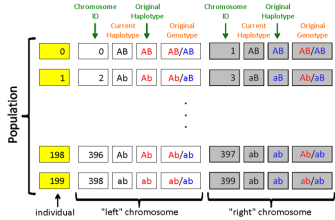
Building the Starting Population
After a user enters all of his or her preferred settings into EvolGenius, the simulation builds the starting population. This is done at the start of each iteration. For each of the N individuals, the following information is stored in the computer's memory:
(1) Two chromosomal haplotypes. These can be AB, Ab, aB or ab.
(2) ID numbers for each chromosome. For the first individual, the chromosomes are assigned ID numbers 0 and 1; these numbers are also assigned to each of the genes on that chromosome. For the second individual, the ID numbers are 2 and 3. For the last individual, these numbers are 2N-2 and 2N-1, where N is the fixed population size.
(3) Copies of the chromosomal haplotypes associated with each ID number, along with the diploid genotype associated with each ID number. For example, if the first individual has the AB/ab genotype, this genotype will be associated with ID numbers 0 and 1.
The rationale for items 2 and 3 will become clear in the discussion of gene copy fixation. For all but one genotype (AaBb), haplotypes can be assigned to each individual without concern about "phase" - that is, how the alleles of the Alpha gene are paired with alleles of the Beta gene. For example, if the individual has the Aabb genotype, we know that one chromosomal haplotype is Ab and the other is ab. However, when the individual has the AaBb genotype, there are two possible ways to phase the alleles: AB/ab or Ab/aB. The simulation assumes that these possibilities are equally likely. Thus, a random number is drawn between 0 and 1, with AB/ab assigned when the random number is less than 0.5, and Ab/aB assigned otherwise.
Figure 1 summarizes a possible starting population where N equals 200; note that the first individual is number 0 and the last is number 199. In this example, for individual 1 (the second individual in the population), the A and b alleles on the first ("left") chromosome are assigned ID #2, while the a and B alleles on the second ("right") chromosome are assigned ID #3.
Reproduction
Choosing Parents
To choose a parent, EvolGenius draws a random number between 0 and 1. This is multiplied by N and rounded down to the closest integer. For example, if N is 150 and the random number is 0.051 (as noted earlier, the resolution is much greater), the product is 7.65, so individual 7 will be chosen. This process is then repeated to choose the second parent. Thus, two individuals are chosen at random to mate; this is common assumption of population genetics models.
If self-mating is not permitted, the second parent is rejected should the two numbers match. In this case, the simulation repeats the process (as many times as necessary) to choose the second parent. If monogamy is enforced, once a mating pair has been created (e.g., individuals 2 and 31), neither individual can be paired with a different individual in a subsequent mating; if either is chosen in a subsequent mating, the original mate is automatically assigned.
Natural Selection
If the relative fitness of a chosen parent's genotype is less than 1, a natural selection test is performed. A random number between 0 and 1 is drawn. If this number is less than the parent's fitness, the parent is retained; otherwise, the parent is rejected. For example, if the parent's fitness is 0.9, the parent will be retained if the random number is 0.4, but the parent will be rejected if the random number is 0.92. Because the random numbers are uniformly distributed, there is a 90% chance that the parent will be retained and a 10% chance that the parent will be rejected. If the parent is rejected, another is chosen at random and subjected to the natural selection test; this is repeated as often as necessary until an individual is retained.
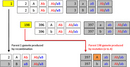
Mating Preference
If all mating (with respect to the Alpha genotype) is equally permissible, then mating will proceed once two parents are chosen. However, if EvolGenius is set for unequal mating preference, a mating test must be performed before mating is permitted. A random number is drawn between 0 and 1. If this number is lower than the mating preference value, then the mating is permitted; otherwise, it is rejected and the full process of picking two parents is repeated. For example, consider the settings in Figure 2. If the two chosen parents happen to have the AaBB and AAbb genotypes, the mating is automatically permitted. However, if the parents are AaBB and aaBb, the mating test is performed; if the random number is less than 0.4, the mating is permitted.
Producing Offspring
Once a pair of parents is chosen (i.e., selection and mating tests, if relevant, are passed), a chromosome from each parent is chosen at random and, behaving like a gamete, is placed into an offspring. For each parent, a random number is drawn between 0 and 1. If this number is less than 0.5, the first ("left") chromosome is used; otherwise, the second ("right") chromosome is used. This is the first step.
This is complicated slightly if the linkage map distance between Alpha and Beta is greater than 0 cM. In this case, a crossover test must be performed. Here, a random number is drawn between 0 and 1. If this number is less than the map distance in cM divided by 100 (e.g., if the map distance is 30 cM, the boundary value is 0.3), crossing-over occurs. Thus, if an individual has the Ab/aB genotype, crossing-over would change this to AB/ab.
Note that the parent's genotype does not change; rather, the genotype changes in the diploid cell that undergoes meiosis. A parent can be involved in more than one mating event, and crossing-over will happen independently in each event (with the same probability of map distance divided by 100). A summary of the possible gametes produced by an individual is shown in Figure 3.
If the user has permitted mutation within an EvolGenius simulation, it will occur during offspring production, essentially in the diploid cell that produces the gamete. Once the gamete haplotype is determined, it is subjected to a mutation test for each gene. A random number is drawn between 0 and 1. If this number is less than the mutation rate of the original allele to the other allele, then mutation occurs. Imagine, for example, that the Ab haplotype is chosen, that the mutation rate of A to a is 0.001, and that the mutation rate of b to B is 0.0002. Two mutation tests are performed, the first to determine if A will mutate to a (there is a 0.1% chance that this will occur), and the second to determine if b will mutate to B (there is a 0.02% chance that this will occur).
It is very important to recognize that the use of upper and lower cases carries no meaning, aside from distinguishing the two alleles of a gene. There are no explicit phenotypes associated with the Alpha and Beta genes. Dominance and/or epistasis can only be specified by setting relative fitnesses. For example, if aa and Aa are assigned relative fitnesses of 1.0, while AA has a relative fitness of 0.9, the a allele is dominant to the A allele. If alleles do affect fitness, it can be assumed that they represent different functional versions of the gene. However, in this simulation, there can only be two functionally distinct alleles. If one allele mutates to the other, all that can be assumed is that the mutation has produced a particular functional version of the gene - one shared by all other copies of the gene represented by a particular letter.
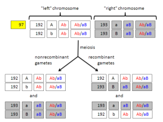
Keeping Track of Allele IDs and Associated Information
Now consider the case where individuals 1 and 198 are chosen as mates. Figure 4 shows how information is passed to offspring, depending on recombination and/or mutation.
When these two gametes are combined, the offspring would have the AB/Ab genotype. It would be stored in the offspring population data set as shown in Figure 5. Thus, when an offspring is produced, the ancestral IDs, along with ancestral chromosomal haplotypes and genotypes, are passed along.
Building a New Generation
Quite simply, EvolGenius repeats the processes described above as many times as necessary to produce a new generation of N individuals. A single offspring will be produced each time a mating is permitted. Parents can be chosen multiple times, and they will be subjected to natural selection and mating tests when required by the simulation settings for relative fitness and mating preferences, respectively. Crossing-over and mutation tests will also be performed when required by the simulation settings. As shown in Figure 5, every time an offspring is produced, the ancestral IDs, haplotypes, and genotypes are stored for all four alleles in its diploid genotype.
Migration
If immigration is permitted, the EvolGenius simulation runs a little differently. First, the information associated with the individuals in the starting population is ignored. This is because the immigrants lack such information (e.g., allele IDs, ancestral haplotypes, and ancestral genotypes), so downstream analyses that use such information cannot be performed.
Immigrants are brought into the next generation before reproduction occurs. If the user has set the average number of immigrants per generation to Ni, then the probability that any given individual in the next generation is an immigrant is Ni/N. Because the simulation maintains a population of constant size, Ni cannot exceed N. The simulation draws N random numbers between 0 and 1. Every time the random number falls below Ni/N, an immigrant is brought into the population. When this occurs, a second random number between 0 and 1 is drawn. This determines the genotype of the immigrant. Table 1 shows how this is done for a population with arbitrary genotype frequencies.
| Table 1. Choosing the genotype of an immigrant. | |||
| Genotype | Proportion of immigrant population | Cumulative proportion of immigrant population | Range of random numbers to choose individual with this genotype |
| AB/AB | 0.0625 | 0.0625 | 0.0000 ≤ r.n. < 0.0625 |
| AB/Ab | 0.1250 | 0.1875 | 0.0625 ≤ r.n. < 0.1875 |
| Ab/Ab | 0.0625 | 0.2500 | 0.1875 ≤ r.n. < 0.2500 |
| AB/aB | 0.1250 | 0.3750 | 0.2500 ≤ r.n. < 0.3750 |
| AB/ab or Ab/aB * | 0.2500 | 0.6250 | 0.3750 ≤ r.n. < 0.6250 |
| AB/ab | 0.1250 | 0.7500 | 0.6250 ≤ r.n. < 0.7500 |
| aB/aB | 0.0625 | 0.8125 | 0.7500 ≤ r.n. < 0.8125 |
| aB/ab | 0.1250 | 0.9375 | 0.8125 ≤ r.n. < 0.9375 |
| ab/ab | 0.0625 | 1.0000 | 0.9375 ≤ r.n. < 1.0000 |
| * Because of phase ambiguity, if an individual has the AaBb genotype, a random number is drawn between 0 and 1; if it is less than 0.5, the immigrant will have the AB/ab genotype; otherwise, the immigrant will have the Ab/aB genotype. | |||
Tracking Allele Frequencies and Allele Fixation
After each new generation is built, the relative frequencies of the A, a, B, and b alleles are calculated directly. If the relative frequency of an allele reaches 1.0 (so the other allele has a relative frequency of 0.0), then allele fixation has occurred; the generation that this occurs for each gene (if it occurs) is recorded. By default, if the population began with one allele at a frequency of 1.0, then fixation is reported to occur at 0 generations.
Say, however, that the user wants to know how long it takes for a favored allele to fix if it was not present at generation 0. The program can be set to only report allele fixation when that particular allele has fixed. Thus, if the population begins with only AA individuals, but A is permitted to mutate to a, the user can set the program to report when the a allele reaches a frequency of 1.0.
By default, the program will run for 30,000 generations or until alleles have fixed for both genes, whichever comes first. The maximum number of generations per iteration can be changed, making it so high that an iteration is virtually guaranteed to finish by fixing alleles (rather than by reaching the maximum number of generations). Alternatively, the maximum number of generations can be set to as low as 1, allowing the user to record relative allele frequencies at an arbitrary number of generations. To guarantee this, the user can set the program to ignore allele fixation.
Considerations for Running EvolGenius Efficiently
Obviously, the time that it takes to build a generation will be proportional to N; larger populations take longer to build. Also, every time the program has to generate a random number, run time will increase. Thus, natural selection, mutation, crossing-over, mating preferences, and migration will add to the run time. So will tracking gene copy history. Couple this with the fact that the program is intended to be run with a large number of iterations, it makes sense to minimize the run time of individual iterations - in ways, of course, that do not compromise the aims of the experiment.
- Only allow crossing-over, mutation, natural selection, or nonrandom mating when the experimental aims relate to these.
- If focusing on a single gene, linkage map distance should be set to 0.
- If the user is not interested in gene copy fixation, then tracking of gene copy history should be turned off. While checking for gene copy fixation is not computationally expensive, waiting for gene copy fixation can extend the iteration considerably. This is because, in a constant-N neutral model for an autosomal gene in diploid organisms, average allele fixation times is -4N[p ln p + (1-p) ln (1-p)] (Kimura and Ohta 1969), where p is the relative frequency (ranging from 0 to 1) for one of two alleles. On the other hand, gene copy fixation time is expected to take, on average, 4N generations. The value of -4N[p ln p + (1-p) ln (1-p)] reaches a maximum when p is 0.5 (0.693 × 4N), but drops off considerably when starting allele frequencies diverge (e.g., when p is 0.1, allele fixation takes, on average, 0.325 × 4N generations). Thus, turning off gene copy tracking can reduce run time by 30% or more.
Some Basic Experiments
Probability of Fixation by Genetic Drift of an Allele as a Function of Initial Frequency (Neutral Model)
You probably want to run a large number of iterations at each starting allele frequency, since your estimates of fixation probability will come from the fraction of iterations that fix each allele. [In the ridiculous extreme, if you only ran one iteration, you would infer that one allele - the one that fixed - has a 100% probability of fixation, while the other has a 0% probability of fixation. The estimates are likely to err less, on average, from the true values if sample size (i.e., the number of iterations) is increased.] You are probably not interested in gene copy history.
All genotypes should have a relative fitness of 1, since you are assuming a neutral model. If you are only interested in one gene, set the linkage map distance to 0 cM. There should be no mutation and no migration. Mating preferences should all be left at 1. Tracking of gene copy history should be turned off. Maximum number of generations should be high (at least 10N, but it may as well be 1,000,000!), to ensure that individual iterations don't stop before allele fixation occurs.
The only setting that will change among runs is the composition of the starting population. The easiest way to set allele frequencies is to start with only AABB and AAbb individuals, ignoring the Alpha gene. The relative frequency of the B allele (p) will be NAABB / (NAABB + NAAbb).
Rate of Genetic Drift as a Function of Population Size
You probably want to see how much allele frequencies change from the start after a set number of generations. You are definitely not interested in gene copy history, since gene copy fixation takes, on average, 4N generations, and you will probably be halting each iteration much sooner than that. You probably want a large number of iterations, because you are interested in estimating the standard deviation of the final allele frequencies.
All genotypes should have a relative fitness of 1, since you are assuming a neutral model. If you are only interested in one gene, set the linkage map distance to 0 cM. There should be no mutation and no migration. Mating preferences should all be left at 1. Tracking of gene copy history should be turned off. You will probably be setting the maximum number of generations per iteration to a small number (e.g., 10 generations).
The relative genotype frequencies in the starting population should be the same for all runs. The only thing you should change is N. For example, you could set the population to have a 1:2:1 ratio of AABB:AABb:AAbb, which is at Hardy-Weinberg equilibrium with respect to the Beta gene. The smallest population may have NAABB = 10, NAABb = 20, and NAAbb = 10, for N = 40 individuals. These numbers could then be increased by orders of magnitude (multiples of 10) to explore the effect on standard deviation of increasing population size.
Effect of Selection on Effective Population Size (Ne)
Gene copy fixation is expected to take, on average, 4N generations in a constant-N population with no selection. Anything that increases variance among individuals in reproductive success should decrease Ne. Gene copy fixation time, therefore, provides an estimate of Ne; Ne can be estimated by dividing gene copy fixation time by four. Therefore, a large number of iterations is necessary to obtain a reliable estimate of Ne from average gene copy fixation time, especially because there can be a very large variance among iterations.
Settings depend, in part, on whether you are interested in solely the effect on Ne of the gene subject to selection, or if you are also interested in the Ne of a second, neutral gene. It also depends on how less fit genotypes arise; they could be present at the start (e.g., simulating a change in selection pressures) or they might appear by recurrent mutation. Regardless, mating should be random, and there should be no migration (since tracking of gene copy history is turned off when migration occurs). Linkage map distance should be 0 cM if only the gene subject to selection is of interest. However, a number of interesting experiments involve varying linkage map distance between the gene targeted by selection and a second, neutral gene.
Establishment of Stable Allele Frequency Equilibriums
There are three straightforward ways to establish stable equilibrium allele frequencies as a consequence of opposing forces. First, equilibrium can be due to opposing mutations: A mutates to a at one rate, while a mutates to A at another (or perhaps, the same) rate. However, mutation must occur in both directions to establish an equilibrium. Second, equilibrium can reflect heterozygote advantage. That is, the relative fitnesses of the two homozygotes must be lower than the relative fitness of the heterozygote. Third, equilibrium can reflect a balance of selection and mutation, with selection removing an allele while mutation reintroduces it. Interestingly, the number of iterations needed to get accurate estimates of equilibrium allele frequencies is not very high, because variance across iterations is low.
Generating Instability
There are two easy ways to destabilize populations - that is, to cause alleles to fix rapidly, even without selectively favoring one over the other. The first is heterozygote disadvantage. Here, the heterozygote has a lower relative fitness than either homozygote. Even if both homozygotes have relative fitnesses of 1.0, fixation of one allele or the other will be accelerated. The second way to generate instability is to favor matings of like genotypes over matings of unlike genotypes. Both situations destabilize as soon as one of the homozygotes gains a numerical advantage over the other, even if it's only due to genetic drift. It comes down to the relative probabilities of AA × AA and aa × aa matings. The ratio of AA × AA to aa × aa matings will be NAA2:Naa2 if AA and aa have the same fitness and if both matings are equally permissible. This means that whichever genotype gains a numerical edge will increase that edge exponentially.
Impossible (?) Simulations for EvolGenius
There are many simulations that can be run using the EvolGenius program, even some that seem "impossible." However, a good understanding of how the program works will help you leverage the software in a variety of challenging ways, similar to the examples below.
Simulating Sex-Linkage
To simulate sex-linkage, you first need to make sex chromosomes. This is done by building a population with only AA and Aa individuals. Think of A as an X chromosome and a as a Y chromosome. Mating preferences have to be set as follows: 1 for AA ´ Aa, and 0 for all other pairs. Thus, AA (XX) can only mate with Aa (XY). The Beta gene will be the sex-linked gene. This is done by setting linkage map distance to 0 cM.
Simulating a Population Expansion
EvolGenius always builds a population with N individuals, so it would seem that simulating a population expansion should not be possible. Again, this involves playing with mating preferences and setting the linkage map distance to 0 cM. We're interested in the Beta gene, and we use the Alpha gene to simulate the population flush. First, decide how much the population should increase in size. If you want an x-fold increase, you want x-1 times as many AA as aa individuals; for example, for a 10-fold increase, you may want 450 AA and 50 aa individuals. The aa individuals should be subdivided into the Beta genotypes. Second, set mating preferences to 0 for all combinations except for AA ´ AA and aa ´ aa, which should be set to 1. Finally, set the relative fitness of aaBB, aaBb and aabb to values that are much higher than the relative fitness of AABB. There shouldn't be any individuals with the AABb, AAbb, AaBB, AaBb, or Aabb genotypes.
This is a very unstable situation. The AABB individuals will disappear quickly, because they can only mate with other AABB individuals and because their relative fitness is low. The flush, in fact, is simulated by the extinction of AABB individuals. The rate of the flush can be controlled by changing the relative fitness of AABB, and will be reflected in the Alpha allele fixation time.
Conclusion
This is just a sampling of the types of simulations EvolGenius is capable of running. Because the program is free for all users and has a quick run time in comparison to traditional lab experiments, EvolGenius can be easily integrated into the classroom and help students to learn about the ways in which genes move through multiple generations of a single population.
References and Recommended Reading
Kimura, M. and T. Ohta. The average number of generations until fixation of a mutant gene in a population. Genetics 61, 763-771 (1969)
A link to a downloadable version of the EvolGenius program is available here.