Adaptation and Phenotypic Variance

Of course, in order to fully understand this equation, one must also understand what each subcategory of genetic variance entails. The first subcategory, additive genetic variance, refers to the deviation from the mean phenotype due to inheritance of a particular allele and this allele's relative (to the mean phenotype of the population) effect on phenotype. In contrast, the second subcategory, dominance genetic variance, involves deviation due to interactions between alternative alleles at a specific locus. For example, say that a plant produces white flowers if its genotype is A₁A₁ and red flowers if its genotype is A₂A₂. If there is no dominance deviation or interaction between these alleles, then the A₁A₂ genotype would lead to pink flowers due to expression of both alleles. However, if there is an interaction between the alleles such that their expression is not equal, then the phenotype of the heterozygote (A₁A₂) would not be an approximate midpoint; rather, it would more closely resemble one of the homozygotes (either A₁A₁ or A₂A₂). For instance, if the A₂ allele was dominant to the A₁ allele, then the heterozygote would produce red flowers.

Finally, like dominance variance, the third category of genetic variance—epistatic variance—involves an interaction between alleles; however, in this case, the alleles are associated with different loci. This concept can be illustrated by returning to the flower color example, but this time assuming that a second locus (denoted B) determines whether flower pigment is produced. In this case, the B₁ allele is dominant, and it codes for the production of pigment; an absence of pigment means that a plant's flowers will be white. Thus, if the plant's genotype is either B₁B₁ or B₁B₂, its flower color will be determined by the genotype at the A locus. On the other hand, if the plant's genotype is B₂B₂, then no pigment is produced, so the flower color is always white and is not influenced by the genotype at the A locus.

Once researchers have determined the total amount of genetic variation responsible for a trait, they can use this information in calculations of the trait's heritability. Heritability is a measure of the proportion of phenotypic variance attributable to genetic variance, and it is an important predictor of the degree to which a population can respond to artificial or natural selection.

Consider, for example, a study involving the rare plant Scabiosa canescens that was conducted by researcher Patrik Waldmann in 2001. Like many rare species, this plant is often found in populations of very small size. Such populations are expected to have a low level of genetic diversity, which would limit their ability to adapt. In his study, Waldmann used genetic lines of S. canescens from both a small and a large natural population to estimate both additive and dominance genetic variation. However, contrary to expectations, Waldmann did not find a lower level of additive genetic variance in the offspring from the smaller population. This finding meant that the smaller population still had the ability to evolve, even though the population consisted of only 25 individuals.

Figure 1: The reaction norm.

Distinct genotypes are represented by variously colored lines. Genotypes in figure 1A respond similarly to steady change in water availability, while genotypes in 1B exhibit a variable responce. The (hypothetical) species in 1B is, therefore, more suited to adapt to environmental change.

© 2008 Nature Education All rights reserved.

Figure Detail

Again, a closer understanding of each of the aforementioned subcategories is critical to an accurate interpretation of the concept of environmental variance. Here, specific environmental variance refers to the deviation from the population mean due to the environmental conditions that are uniquely experienced by each individual. Statistically speaking, this is called the error or residual variance. From the perspective of a plant or animal breeder, specific environmental variance is basically random noise in the expression of the true phenotype, and it can interfere with artificial selection of traits of commercial interest by weakening the correlation between genotype and phenotype.

The second subcategory of environmental variance, general environmental variance, is attributed to the nongenetic sources of variation between individuals that are experienced by multiple individuals in a population. This is typically the largest component of variance in populations in natural conditions. While specific environmental variance is determined by the variation within replicated genetic lines, to obtain an estimate of general environmental variance, replicates of each of the genetic lines need to be assessed in each natural or experimental environment of interest (Fisher et al., 2004; Merilä et al., 2004). If just one environmental treatment is used, then all nongenetic sources of variation are due to the specific environment (i.e., the different microenvironments of individuals).

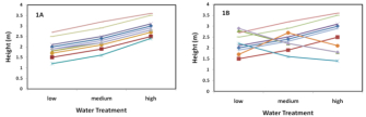
Estimates of general environmental variance can be determined by growing or raising the same set of genetic lines in all environments of interest. For example, water is required for all plants, but the amount that promotes maximum growth differs among both species and genetic lines of a species. Consider an experiment that grows 10 genetic lines of corn in each of three levels of soil moisture (low, medium, and high). On average, the genetic lines grow slower in the low and high moisture soils as compared to the medium moisture soil. Here, the changes in growth rate due to the different water treatments are equal to the general environmental variance. In Figure 1A (called a reaction norm), where the different lines represent different genotypes, the change in height (estimate of growth rate) associated with the different watering treatments illustrates the environmental variance.

Finally, the third subcategory of environmental variance—genotype by environment interaction—involves the unique or different responses of genetic lines to general environmental variation. To better understand this concept, once again consider the corn grown in different water levels. Among the 10 genetic lines under study, the response to water availability may not be parallel. For instance, some genetic lines may be less negatively affected by low or excessive moisture levels. Returning to Figure 1A, notice the similar response to greater water availability across all genotypes. In this case, there is no genotype by environment interaction, as all of the genotypes have a similar response to the same environmental change. However, in Figure 1B, the lines cross, which indicates that the different genotypes have different responses to an identical change in water availability. This differential response to environmental change (or genotype by environment interaction) can contribute to a species' ability to be successful in heterogeneous environments (Barrett et al., 2005).

Both general environmental variance and genotype by environment interaction are aspects of a characteristic known as phenotypic plasticity. Phenotypic plasticity is a change in the phenotype associated with a given genotype in response to different environmental conditions. Some researchers believe that genotype by environment interaction provides the best estimate of the potential for phenotypic plasticity to evolve. Other researchers argue that the correlation of genotype expression across two environments is a better indicator of this potential (Via & Hawthorne, 2005).