Characterizing Communities

A community is a group of interacting species that inhabit a particular location at a particular time. Community ecologists study the number of species in a particular location and ask why the number of species changes over time. They also study communities in different locations, and ask why the number of species differs with location.

Community ecologists often study a narrow group of species. For example, a community ecologist who studies stream fishes may study the fishes that occur in small streams. Another community ecologist may study parasites of sharks. These narrower communities are defined as assemblages, species that share an attribute of habitat or taxonomic similarity, or taxon.

Multiple communities might be spread across an area. An interesting question becomes, why do the communities not have the same numbers of species or the same abundances of species? Comparisons can be made among communities using attributes such as species richness, species diversity, and evenness. Species richness is simply the number of species in a community. Species diversity is more complex, and includes a measure of the number of species in a community, and a measure of the abundance of each species. Species diversity is usually described by an index, such as Shannon’s Index H'. Species evenness is a description of the distribution of abundance across the species in a community. Species evenness is highest when all species in a sample have the same abundance. Evenness approaches zero as relative abundances vary. Species evenness can also be described using indices, such as the J' of Pielou (1975). Figure 1 is a simple diagram to describe species richness and species evenness. All diversity indices are criticized because they combine the number of species and the relative species abundances for one area into a single index, confounding these variables (Ludwig & Reynolds 1988).

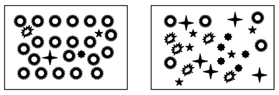
Figure 1: Species evenness and species richness for animalcule communities

Both communities contain five species of animalcules. Species richness is the same. The community on the left is dominated by one of the species. The community on the right has equal proportions of each species. Evenness is higher when species are present in similar proportions. Thus the community on the left has higher species diversity, because evenness is higher.

Three levels of diversity have been studied by community ecologists. Alpha diversity is within-habitat diversity. Beta diversity is between-habitat diversity. This refers to changes in diversity along an environmental gradient. Gamma diversity or large-scale landscape diversity combines alpha diversity and beta diversity.

Comparison of these community attributes is not as simple as it may appear. For example the number of species that are detected in a community may depend on the number of samples collected. Higher numbers of species are collected with an increased number of collection samples. This invalidates comparisons if the number of individuals collected differs among collections. A solution to this predicament is to standardize the sampling effort by creating a taxon sampling curve. Gotelli & Colwell (2001) described the use of sampling curves, such as rarefaction, to compare taxon (species) richness among samples. Rarefaction is a Monte Carlo resampling approach to develop a curve to identify and allow comparisons among samples using the minimum sample size of all the collections.

Species diversity tends to increase with habitat heterogeneity. Communities that have increased habitat variation have an increased number of ways to divide up the available niches. The number or variation of available niches varies by organism-type. Plant niches tend to be defined by different variables than animal niches. Plant species richness may vary with variation in local soil properties. Animal species richness may vary with the complexity of the habitat form, for example vegetation structure. Thus habitat heterogeneity is both context and species dependent.

An obvious pattern of communities is the variation in species abundances. Abundance patterns in communities can be examined by numbers of individuals per species, biomass per species, or percent cover per species. The most common approach is to examine numbers of individuals per species to create a frequency distribution. Abundance patterns of species in communities have some predictability. Most species in a community tend to have intermediate abundance levels. A few tend to be extremely common, and a few are rare. The shape of this distribution fits the predicted pattern with an increased number of sample collections. The distribution of abundance in communities can be described by a lognormal curve (Preston 1948). For example, Figure 2 depicts the abundances, or number of individuals, for fish species collected in the Wabash River during a 25-year period.

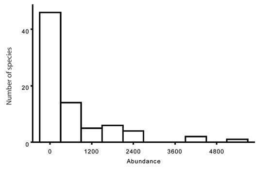
Figure 2: Abundances of fish species in the Wabash River

The abundances of fish species that were collected in the Wabash River from 1974-1998. The majority of species occurred in low abundance, and a few species were extremely abundant. Data are from Pyron et al. 2006.

Comparisons among communities frequently result in patterns of species that coexist, or species that tend not to coexist. A potential explanation for patterns of why species do not coexist is competition. This may be observed if two species tend to occur in similar communities, but never occur together in a single community. If the two species use similar resources they have overlapping niches. Studies of niche overlap can be for resources of food, habitats, or timing for use of habitats. An example of two species with similar niches, and that do not occur together are the redfin shiner and the Ouachita Mountain shiner in the Little River watershed of Oklahoma and Arkansas. Both species are small minnows that inhabit rocky pools in small to medium streams, and consume aquatic macroinvertebrates. Taylor & Lienesch studied the distribution of the species at 65 stream sites and found the Ouachita Mountain shiner at 35 sites, redfin shiner at 30 sites, and only one site with both species present. Although the mechanism for creating the distribution pattern cannot be determined, Taylor & Lienesch concluded that competition likely maintains their segregation.

Food webs describe the trophic, or feeding relationships among the members of a community. Trophic relationships refer to where and how organisms obtain their energy. For example, primary producers are organisms that convert energy from light or heat into organic tissue. Plants are an example of a primary producer. Consumers are organisms that get their energy from eating primary producers. A rabbit is a consumer that eats grasses. Predators are organisms that eat consumers. A wolf is a predator that eats rabbits. Food webs can be simple or they can be complex, depending upon the number of species in a community. Food webs can vary in complexity by the number of connections between member species.

Spatial and temporal comparisons of communities provide information about the things that cause differences in species occurrence and abundance patterns. A spatial comparison refers to comparing similar communities that occur in different locations. This allows an ecologist to test if there are differences in climate, landscape features, geology, or habitats that occur with different species assemblages. For example, in small streams, the fish species that occur in a riffle habitat (stream location with change in height of the stream bottom) tend to be different than the fish species that occur in pool habitats (stream location with constant stream bottom height). In other words the fish assemblages of riffles differ from the fish assemblages of pools. The assemblage differences are largely due to the fact that the habitats are so different. Riffles have higher gradients, increased flows, and larger substrates than the pool habitats of streams. At a larger scale, fish assemblages in larger rivers differ from fish assemblages in small streams.

A temporal comparison refers to comparing the same community at different times. The species composition of communities and assemblages changes with time. Change may occur following disturbance events, or change may occur due to stochasticity in assemblages. The predictable change that occurs to assemblages in the context of a natural disturbance regimen, is frequently interpreted as succession.

Communities can be characterized by natural disturbance regimes. Disturbance events are characterized by their frequency and impact. Disturbances can include variation in climate, variation in flooding frequency or drought frequency, or frequencies of storm events. Species have adaptations that were shaped by exposure to natural disturbance regimes during their evolutionary history. For example, insects that occur in temperate headwater streams frequently have life history adaptations that result in larval stages being present during the season when leaf inputs from terrestrial plants are high. Insects that occur in desert streams might have adaptations for surviving unpredictable flood events.

The life histories of organisms are a product of their local environment, including the predictability of disturbance regimes. Organisms can be classified in three general life history modes. Winemiller & Rose (1992) classified fishes based on three life history variables: juvenile survivorship, number of offspring, and age of maturity. An interesting product of this classification exercise was that species in these three groups differ in their ability to survive disturbances. For example, fish species with low juvenile survivorship, low number of offspring, and with early maturity tend to be successful in habitats with unpredictable droughts or floods. Species with a different suite of life history traits such as low juvenile survivorship, high number of offspring, and late maturity cannot survive unpredictable flood or drought disturbances.