Abstract
The rapid development of next generation sequencing (NGS) technology provides a new chance to extend the scale and resolution of genomic research. How to efficiently map millions of short reads to the reference genome and how to make accurate SNP calls are two major challenges in taking full advantage of NGS. In this article, we reviewed the current software tools for mapping and SNP calling and evaluated their performance on samples from The Cancer Genome Atlas (TCGA) project. We found that BWA and Bowtie are better than the other alignment tools in comprehensive performance for Illumina platform, while NovoalignCS showed the best overall performance for SOLiD. Furthermore, we showed that next-generation sequencing platform has significantly lower coverage and poorer SNP-calling performance in the CpG islands, promoter and 5′-UTR regions of the genome. NGS experiments targeting for these regions should have higher sequencing depth than the normal genomic region.
Introduction
The advent of Next Generation Sequencing (NGS) technology has significantly advanced the sequence-based genomic research and its downstream applications1 which include, but not limit to, metagenomics, epigenetics, gene expression, RNA splicing and RNA-seq and ChIP-seq2,3. In the past three decades, the Sanger method4 has been applied in many significant large-scale sequencing projects and is considered as a ‘gold standard’ because of its appropriate read length and high accuracy5. So far, three NGS platforms, the Roche/454 GS FLX, the Illumina/Solexa Genome Analyzer and the Applied Biosystems SOLiD System, have attained world-wide popularity. NGS focuses on generating three to four orders of magnitude more sequences but with considerably less cost in comparison with the Sanger method on the ABI 3730xL platform (hereafter referred to as ABI Sanger)5,6,7. Despite the recent advances of NGS technologies, it is not clear whether the sequencing coverage by the NGS is the same across different regions of the genome.
After the short reads are generated, the first step is to align them to the reference genome. To discover tumor genetic information through resequencing different control/case samples, the mapping process must be able to efficiently align millions of sequences generated. Alignment algorithms should be robust enough to sequencing errors, but be able to detect true genomic polymorphisms2. To take full advantage of NGS, more and more efficient algorithms are designed to overcome the limitation of read length and non-uniform error score in NGS data.
Because of the tremendous volume of reads and the huge size of the whole reference genome, alignment speed and memory usage are the two bottlenecks in mapping NGS reads. Traditional algorithms, such as BLAST8 and BLAT9, can perform the NGS alignment more precisely, but they usually take a few days even on computer grids, not to mention personal computers. The time and cost are usually unaffordable for most biologists. Another challenge is how to pick true hit from multiple hits. Generally many aligners will report all possible locations with the appropriate tags or pick a location heuristically. If the multiple hits cannot be ranked for certain standard, it will make the comparison between read and reference unreliable. Furthermore, since the sequencing genome is usually different from the reference genome, alignment algorithms should be robust enough to sequencing errors, but do not miss true genomic polymorphisms2. To handle these challenges, a lot of short-read alignment programs have been developed in recent years. A brief review of the popular programs is provided in supplementary materials and all of them are free for academic and non-commercial use.
Based on the core alignment techniques used, the programs can be classified into three categories10,11. The first category uses hashing tables and it can be further divided into two sub categories, either hashing the reads then using the reference genome to scan the hash table, such as RMAP12,13, MAQ14, ZOOM15, SeqMap16, SHRiMP17 (for the updated version 2, it hashes the genome18) and RazerS19, or hashing the reference genome then using the set of input reads to scan the hash table, such as MOM20, Novoalign, MOSAIK and BFAST21. (‘Hash table’ refers to a common data structure that is able to index complex and non-sequential data in a way that facilitates rapid searching.)
The second category of programs, such as Bowtie22 (which does not support gaps yet), BWA11,23 and SOAPv224, are based on the Burrows–Wheeler Transform (BWT)25. They can efficiently align short sequencing reads against a large reference sequence, allowing mismatches and gaps. These methods typically use the FM index data structure, proposed by Ferragina and Manzini, who introduced the concept that a suffix array is much more efficient if it is created from the BWT sequence, rather than from the original sequence26. The FM index retains the suffix array's ability for quick pattern search and is generally smaller than the input genome size27.
The third category is implemented by merge-sorting the reference subsequences and read sequences. The representative one in this category is Slider28, which is focused on the Illumina platform data. The characteristics of the chosen software and their output formats are summarized in Table 1. Since the first two categories are predominately used, we have assessed the performance of the representative software in the two categories.
Furthermore, accurate alignment is not sufficient to meet the needs of further scientific discovery for most resequencing projects. For example, the 1000 Genomes Project aims at sequencing more than 1000 human genomes to characterize the pattern of genetic variants (common and rare) (http://www.1000genomes.org/). TCGA (http://cancergenome.nih.gov/) has been sequencing a large number of cancer and normal samples for different individuals, targeting at the genetic variations of tumor. To this end, the whole analysis pipeline should also include detecting genomic variations including single nucleotide polymorphism (SNP), copy number variations (CNV), inversions and other rearrangements29. Although NGS provides a sequencing error score, it is hard to distinguish true genetic variation from the sequencing error or mapping error30.
Currently, there are several methods available for calling SNPs from NGS data, including Pyrobayes31, PolyBayes32, MAQ14, SOAPsnp33, Varscan34, SNVMix35,36, SeqEM37 and Atlas-SNP229. Pyrobayes and PolyBayes recalibrate base calling from raw data and then implement a Bayesian approach that incorporates prior information with population mutation rates to detect SNP. MAQ derives genotype calls from a Bayesian statistical model that incorporates the mapping qualities. It measures the confidence that a read actually comes from the position it aligns to, error probabilities from the raw sequence quality scores, sampling of the two haplotypes and an empirical model for correlated errors at a site. SOAPsnp is also based on the Bayes' theorem. It first recalibrates the sequencing quality score to calculate the likelihood of genotype for each position with existing conversion matrix and then combines the prior probability for each genotype to infer the true genotype33. Varscan uses parameters such as the overall coverage, the number of supporting reads, average base quality and the number of strands observed for each allele to predict genotypes34. SNVMix combines three Binomial mixture models to model allelic counts, nucleotide and mapping qualities of the reads and infers SNPs and model parameters with the expectation maximization (EM) algorithm36. In contrast, SeqEM estimates parameters in an adaptive way. It uses the EM algorithm to numerically maximize the observed data likelihood with respect to genotype frequencies and the nucleotide-read error rate based on the NGS data of multiple unrelated individuals37. Atlas-SNP is similar to SOAPsnp, but it infers systematic errors of base substitutions on single reads by fitting training datasets using a logistic regression model which identified read sequence-related covariates to the base-quality score29.
We used three representative programs – MAQ(version 0.71), SOAPsnp(version 1.03) and SNVmix(version 2-0.11.8-r4)- to call SNP on the merged GBM alignment result in bam file format38 and assumed the genotype of each base to be in one of three states: ‘aa’ as homozygous for the reference allele, ‘ab’ as heterozygous and ‘bb’ as homozygous for the non-reference allele, with the latter two genotypes constituting an SNP36. We compared the NGS analysis result with the SNPs detected by the Affymetrix genome-wide human SNP array 6.0, which was treated as the gold standard. According to the setting, a true positive SNP is a site whose genotype is called as ‘ab’ or ‘bb’ in array and a true negative SNP is ‘aa’.
Results
Alignment performance
We evaluated the performance of sequence mapping software in aligning reads from the cancer genome atlas (TCGA) project39, including 2 × 13,326,195 paired-end reads (SRR018643) and 15,578,118 single-end reads (SRR018725) with length of 76bp each from the Glioblastoma multiforme (GBM) sample (SRS004141) sequenced on Illumina Genome Analyzer II, 2 × 13,716,752 paired-end reads (SRR018658) with length of 76bp each from blood derived normal sample (SRS004142) sequenced on Illumina Genome Analyzer II and one million single-end reads(SRR030482) with length of 50bp from the Serous Cystadenocarcinoma sample (SRS004260) sequenced on the AB SOLiD System 3.0.(see Method section for detail)
To compare the aligner performance fairly, we adjusted the parameters of each exact match programs to standardize the general filters: at most 5 mismatches in whole read or at most 2 mismatched in first 28 bases seed region (if supported. Consider average 10% error base calling rate in 30bp 3′bp tail and basic 2-seed-mismatch maq-like policy). However, this filtering strategy does not fit well for Smith-Waterman based algorithms. Smith-Waterman based algorithms penalize all errors (insertion, deletion, mismatch, etc) quantitatively and summarize them into one mapping score for filtering. And if encountered with paired-end reads, the insert range should be set from 0bp to 1,000bp. The setting for insert size is a very loose standard because the insert size for our pair-end sample in the genomic library has an average length of 586bp with a standard deviation of 101bp. Default settings were used for the other parameters of each program.
From previous experiments, input/output loads were not significant factors in total running time22, so only CPU time was considered for assessment. We also divided the CPU running time into two parts, time for index and time for alignment. Because the index is reusable, the expensive cost of indexing will no longer exist in the application afterwards. We tested these software tools on a typical desktop workstation with a 2.66 GHz Intel core 2 processor Q9400 and 16GB of RAM and the system openSUSE 11.1. All programs run on a single thread.
The assessment results based on Illumina paired-end data are summarized in Table 2. BWT based aligners, Bowtie and BWA demonstrated the best overall performance compared with other index based methods. Bowtie has balanced alignment sensitivity, efficient CPU usage and memory consumption, finishing the job within two and half hours with over 67.5% reads aligned. Compared with Bowtie, BWA needed 88% more time to do the alignment but with only 5% more reads aligned (72.99%) in 2-seed-mismatch maq-like policy.
RMAP, ZOOM and Maq belong to the “hashing reads” category. Due to the huge volume of reads to deal with, their memory footprints are not flexible anymore, ranging from 8GB to 10GB, which may not be feasible for non-expert users. ZOOM beats the other “hashing reads” aligners significantly, using 7 hr to complete alignment with 60% sensitivity. Maq reached a better sensitivity of 72.0%, but consumed 39 hr 10 min for alignment. Thus the alignment speed up by nearly 20 folds in bowtie than Maq for 76bp length reads and the Maq also got a slighter higher sensitivity than bowtie, which is consistent with the comparison in bowtie paper22. For the “hashing reference” aligners tested, as expected, they had the worst performance on the running time and memory consumption when parallelized computing was not implemented; however, due to the underlying Needleman-Wunsch (Novoalign) and Smith-Waterman (SHRiMP) exact search algorithms, they showed excellent sensitivity. SHRiMP had a sensitivity of 81.2%, which was nearly 20% higher than Bowtie, but it took 100 times longer than Bowtie for alignment due to the thread and RAM limitation. We also evaluated the performance of the eight programs on Illumina single-end data from the same GBM sample ( Supplementary Table 1 ) and observed similar results. To validate that the sample phenotype does not affect the performance of the aligner, we tested one run from normal sample ( Supplementary Table 2 ), the relative rankings of memory consumption and computing speed of each aligner are similar in both samples. Meanwhile, the differences on sensitivity in both samples also have the similar trends for all aligners, which should be attributed to the heterogeneity of sample inner property and the variation in the sample amplification stage.
For the SOLiD data, NovoalignCS showed the best overall performance. Different from the letter-space index, all aligners except ZOOM create color-space index for SOLiD data. On average they had a lower proportion of reads mapped compared with the Illumina data. The time for the extremely high sensitivity in SOLiD alignment of SHRiMP was more than 1000 times longer than Bowtie ( Supplementary Table 3 ).
The preferred output format for each program is also listed in Table 1. The Sequence Alignment/Map (SAM) format38 is designed to support both single and paired-end reads, including color space and base space reads from different platforms, which creates a well-defined interface between alignment and downstream analysis.
Sequencing depth, CpG islands and genomic coverage
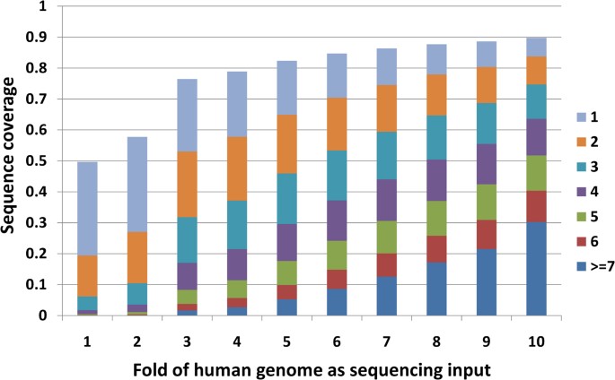
We investigated how many sequencing depths are required to cover the whole genome. We mapped 13 runs of the GBM sample SRS004141 in experiment SRX006310 to the reference human genome (UCSC genome browser human genome version hg18) with Bowtie. With the increase of sequencing depth, the percent of genome covered increases (Figure 1). At one fold sequencing coverage (1 fold coverage = human genome 3.0 gigabases), only less than 50% of the genome was covered at least once and less than 20% was covered at least twice. At ten folds sequence coverage, nearly 90% of whole genome was covered and 83% was covered at least twice.
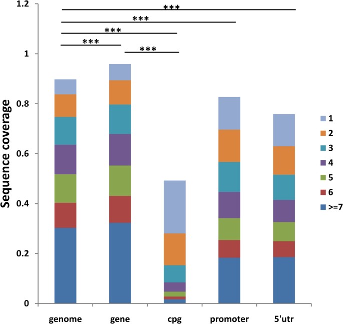
We next investigated whether different genomic regions have different coverage. We found CpG island regions have significant lower coverage than the whole genome and gene regions (both P values less than 2.2e-16). At ten folds coverage, only 50% of CpG islands were covered at least once, compared to 90% for the whole genome (Figure 2). Similarly, at one fold coverage, the numbers are 20% and 50% respectively ( Supplementary Figure 1 ).
Coverage comparisons for different genetic regions at ten folds coverage.
P-value (all are less than 2.2e-16) for t-test through bootstrap shows the significant poorer coverage of CpG-island region compared with genomic background or gene region. Meanwhile, the promoter and 5′UTR region are both significantly under-covered. (One star: p-value<0.05, two stars: p-value<0.01, three stars: p-value<0.001).
Since CpG islands are in 74% of upstream promoters and 40% of the downstream promoters of mammalian genes40, we hypothesized that, the promoter and 5′UTR regions, which are important for regulatory roles of the genome, are also under covered by the NGS technology. Indeed, in all three folds we tested, promoter and 5′UTR regions are significantly under covered by next generation sequencing when compared with whole genome background ( Supplementary Figure 2 ) (both P values less than 2.2e-16). At ten folds coverage, only 83% promoter and 76% 5′UTR regions were covered at least once, compared to 90% for whole genome. The numbers are 42%, 40% and 50% respectively at one fold coverage.
Although gene region is well known to have a higher GC-content than the genome average, its coverage, unlike CpG-island, is higher than the genome average. To further study the relationship between GC-content and sequence coverage, we randomly picked 10,000 windows with 1kb length each from human genome and computed their GC-content and sequence coverage at 10 fold coverage. We observed that sequence coverage increases with GC-content increase when GC-content is less than 40–45%, but decreases when GC-content is more than 50–55%, with the peak at around 45% ( Supplementary Figure 3 ). This observation is consistent with previous discovery41. The CpG island, promoter and 5′UTR regions have average GC-contents of 68.6%, 57.7% and 51.1%, which are higher than the peak at GC-content of 45%. This explains why all of them have sequence coverage lower than the genomic average. On the contrary, the gene region has average GC-content of 46%, which is at the peak. The figure explains why the coverage in that region is higher than whole genome average (with average GC-content of 41%).
We then investigated whether the repetitive element is also a factor causing low mappability in regulatory regions. For total 22571 promoter sequences, we ranked them by repetitive coverage (the portion of the sequence is covered by repetitive element) and then chose top 200 and bottom 200 sequences to compare their coverage pattern. Though the t-test showed significant difference between them (top: 0.94±0.10 (mean ± std), bottom: 0.83±0.21, p-value: 7.33e-12), surprisingly, the sequences enriched for the repetitive element have considerable higher coverage. We further ranked the promoters by GC-content then do the similar test. We found that the top 200 promoters have significantly lower coverage than the bottom 200 promoters (top: 0.10±0.10, bottom: 0.92±0.13, p-value: 1.15e-222). The results indicated that the relatively higher GC-content is the major cause of the lower coverage in regulatory regions.
SNP discovery performance
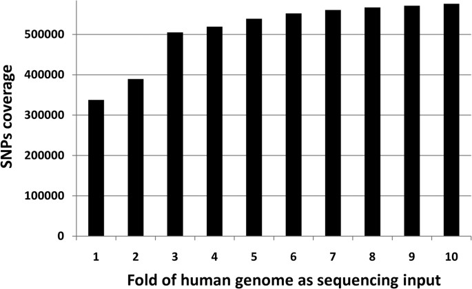
We chose high quality SNP probes as our test set by removing the probes with a confidence score above 0.018. The test set consisted of 583,891 probes, 98% (575,765/583,891) of which were covered by NGS when ten folds coverage were used. The relationship between NGS SNP coverage and genome fold coverage is shown in Figure 3. Under the default setting (SNVmix parameter was first set as same as that used in the original paper for the lobular breast tumor35, then trained itself by the model SNVmix2, which extended original Binomial mixture model SNVmix1. However, the genotype result for self-training parameter showed similar ROC performance, so we applied the first one), we obtained area under the ROC curve (AUC) (see Method). MAQ and SOAPsnp have similar results (AUC (MAQ) = 0.8872, AUC (SOAPsnp) = 0.8866) and both outperform SNVmix significantly (AUC (SNVmix) = 0.8394) (both P-value are < 2.2e-16).
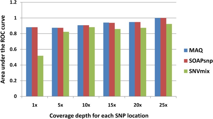
We also studied the SNP calling capability of the three software tools on different depths (Figure 4). Due to the underlying post Bayesian concept, the accuracies of SOAPsnp and MAQ increase as the depth of the target bases increase. However, the SNVmix even demonstrated a worse performance under higher coverage at 21–25 depths, which suggests its unstable performance without the self-training parameters. For low-coverage SNPs, especially with the depth between 1×–10×, the performances of MAQ still remain the best.
Alternatively, we calculated the overall genotype concordance which is defined in VariantEval module of the Genome Analysis Toolkit (GATK)42 to measure the agreement between SNPs called from NGS and array ( Supplementary Figure 4 ). The concordance score was defined as (A+F+L)/ (A+B+C+E+F+G+I+J+L) ( Supplementary Table 4 ). The profile is similar to the AUC measurement, which shows that SNVmix is unstable in high depth situation. The low concordance score when coverage depth is under 20-fold suggests that there is still a big challenge to distinguish the heterozygote from the minor homozygote when sequence coverage is low.
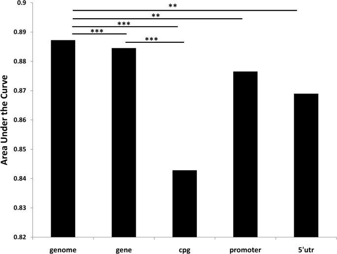
Due to the poor sequence coverage in CpG-island, we tested the classifying performance for 711 SNP probes in array, which are located in CpG-island and covered by merged alignment files. The AUC for each method is, MAQ: 0.8429, SOAPsnp: 0.8379 and SNVmix: 0.5801. We further tested performance for the promoter (3169 SNP probes) and 5′UTR region (1099 SNP probes) ( Supplementary Table 5 ). No matter which classifier was applied, performance in these regions was significantly inferior to the genome background (P-value < 0.01) (Figure 5).
AUC (area under the curve) comparison for different genetic regions.
CpG-island region has significantly poorer performance than genomic background (p-value = 0.000972) or gene region (p-value = 0.0003607). Promoter (p-value = 0.00873) and 5′UTR (p-value = 0.00946) region shows similar pattern. Gene-region also reach a little bit lower performance (p-value = 0.0004641).
Discussion
We have assessed eight representative NGS mapping tools in aligning reads from the cancer genome atlas (TCGA) project. FM-index based aligners with BWT performed best in both paired-end and single-end short reads alignments. Evaluated on reads sequenced on the Illumina Genome Analyzer II, Bowtie demonstrated the best overall performance. Bowtie has balanced alignment sensitivity, efficient CPU usage and memory consumption, finishing one run of sequences on the human genome within 2.5 hours with over 67.5% reads aligned. Meanwhile, we should admit that a lot of aligners can run in muliti-thread mode in practical and hardware limitation may not be the barrier for normal groups. For example, the SHRiMP2 paper compare SHRIMP2, BFAST, BWA and Bowtie's performance on artificial data for different variation cases while utilizing an 8 core 3.0Ghz Intel Xeon machine with 16Gb RAM18. For that case, SHRiMP 2 showed an acceptable speed (20 folds slower than bowtie) and significantly higher precision and recall rate. Thus if we primarily target the highly polymorphic reads and do parallelization, these Smith-Waterman string matching algorithm based aligner should be our first choice in practice.
With bowtie as the aligner, 90% of the whole genome were at least once and 83% were covered at list twice when 10 folds (30 gigabases) input was given. Our results show that 3 folds may be a minimum requirement for input raw data to reach more than 50% of whole genome coverage.
In addition, we found that the CpG-island region shows a significantly poor coverage compared with the whole genome average. The promoter and 5′UTR regions, which harbor regulatory elements and are closely associated with CpG islands40,43, are also significantly under-covered by NGS compared with the whole genome. Thus to discover above regions with target depth, we need to increase the number of runs. For example, to cover 50% of genomic region at least one depth, we need only one fold of the whole genome. However, to cover CpG island regions with the same criteria, we need ten folds of the whole genome ( Supplementary Figure 2 ).
We also evaluated the SNP calling capability of three software tools and found that MAQ performed the best. We found that similar to mapping coverage, SNP calling performance also vary in different genomic regions. The CpG islands, promoter and 5′UTR regions have significantly lower SNP calling performance than the genome and gene body regions. For the SNP analysis, 10 folds input is enough for the standard evaluation, though for the classic Bayesian method, the higher sequencing depth, the more accurate the SNP call will be. We only evaluated the software's capability on detecting known SNPs covered by array, but not on novel ones. Several groups have pioneered in this direction44, but how to evaluate the accuracy is yet to be solved in practice. Due to the limitation of SNP array on the number and distribution of the probes, NGS based GWAS will get a better resolution on the diseases related bio-markers.
In summary, we assessed major NGS analysis tools for sequencing mapping and SNP calling and found that Bowtie is the best tool for mapping and MAQ the test tool for SNP calling. Furthermore, we found that CpG rich regions, such as promoter and 5′UTR, where regulatory elements are usually located, are poorly covered by the NGS platforms. This discovery raises the concerns for NGS technology, particularly when regulatory elements are the focused study regions. NGS experiments for studying these regions should have higher sequencing depth than the normal genomic region.
Methods
Reads extraction
The sequences all in fastq (csfastq for SOLiD) format were extracted from the database of genotype and phenotype (dbGap) in NCBI by sequence read archive (SRA) toolkit. They were then mapped to the human reference genome [NCBI build 36.3] through assigned aligners. The real data was not filtered or modified (besides trimming) from what they originally appeared in SRA.
Coverage comparison for genomic regions
5′utr, 3′utr and gene regions were directly retrieved from refGene table in RefSeq genes track for hg18 through UCSC genome browser. Promoter regions were defined as starting at 5kb upstream of the transcriptional start site, ending at the terminate coordinate of the gene. CpG islands regions were retrieved from cpgIsland table in CpG Islands track for hg18 through UCSC genome browser. The repetitive elements were downloaded from the RepMask 3.2.7 track in UCSC genome browser. Genome background regions were simulated by randomly picking 10000 windows with 1kb length each from hg18 human genome. Each original genomic region entry was in browser extensible data (BED) format. Then we filtered the redundant entry and merged the overlapped entries together for each genomic feature. For each entry, we computed the coverage percentage from the merged NGS alignment files. Then we figured out the average coverage for each genomic feature.
To validate the significance of difference between coverage of different genomic features, firstly we did 1000 times bootstrap to get 1000 sets of coverage entries of each genomic feature (each time with 80% volume of total entry number in the feature category). Then we did two-sided t-test for comparison between two features to get the P-value.
Performance test for the SNP-caller
For SOAPsnp and MAQ, we assigned the Phred-scaled likelihood that the genotype is identical to the reference, which is also called ‘SNP quality’, as predictor and assigned the 1 and 2 genotype in Affymetrix array as SNP case and 0 in genotype as SNP control for the response. We also did the 0 to 2 and 2 to 0 conversion when the minor allele is the reference allele, before ROC display and AUC calculation. SNVmix outputs 3 possibilities, homozygous to reference, heterozygous genotype and homozygous to the non-reference, we added the latter two (AB and BB) together to get the ‘SNP possibility’ as predicator and also assigned the 1 and 2 genotype in Affymetrix array as case and 0 in genotype as control for the response. To provide statistical significance for the comparison between different classifiers, firstly we found the genomic location which is both covered by SNP array and the NGS alignment method (total 583891 in Figure 3), then we did bootstrap 1000 times to get 1000 AUC values for each classifier (each time with 80% volume), lastly we did two sided t-test to get the p-value. To compare the performance of classifier in different regions (the regions for each feature were defined as above), we do the similar: firstly we found those coordinates which located in certain features and both covered by array and NGS alignment, then for each feature, we did bootstrap to get 1000 AUC values from the method, lastly we did the same two sided t-test to compare different features to get the p-value.
References
Flicek, P. & Birney, E. Sense from sequence reads: methods for alignment and assembly (vol 6, pg S6, 2009). Nat Methods 7, 479–479 (2010).
Mardis, E. R. The impact of next-generation sequencing technology on genetics. Trends Genet 24, 133–141 (2008).
Mardis, E. R. Next-generation DNA sequencing methods. Annu Rev Genomics Hum Genet 9, 387–402 (2008).
Sanger, F., Nicklen, S. & Coulson, A. R. DNA sequencing with chain-terminating inhibitors. Proc Natl Acad Sci U S A 74, 5463–5467 (1977).
Bonetta, L. Genome sequencing in the fast lane. Nat Methods 3, 141–147 (2006).
von Bubnoff, A. Next-generation sequencing: the race is on. Cell 132, 721–723 (2008).
Schuster, S. C. Next-generation sequencing transforms today's biology. Nat Methods 5, 16–18 (2008).
Altschul, S. F., Gish, W., Miller, W., Myers, E. W. & Lipman, D. J. Basic Local Alignment Search Tool. J Mol Biol 215, 403–410 (1990).
Kent, W. J. BLAT–the BLAST-like alignment tool. Genome Res 12, 656–664 (2002).
Li, H. & Homer, N. A survey of sequence alignment algorithms for next-generation sequencing. Brief Bioinform 11, 473–483 (2010).
Li, H. & Durbin, R. Fast and accurate short read alignment with Burrows-Wheeler transform. Bioinformatics 25, 1754–1760 (2009).
Smith, A. D., Xuan, Z. Y. & Zhang, M. Q. Using quality scores and longer reads improves accuracy of Solexa read mapping. BMC Bioinformatics 9, 128 (2008).
Smith, A. D. et al. Updates to the RMAP short-read mapping software. Bioinformatics 25, 2841–2842 (2009).
Li, H., Ruan, J. & Durbin, R. Mapping short DNA sequencing reads and calling variants using mapping quality scores. Genome Research 18, 1851–1858 (2008).
Lin, H., Zhang, Z., Zhang, M. Q., Ma, B. & Li, M. ZOOM! Zillions of oligos mapped. Bioinformatics 24, 2431–2437 (2008).
Jiang, H. & Wong, W. H. SeqMap: mapping massive amount of oligonucleotides to the genome. Bioinformatics 24, 2395–2396 (2008).
Rumble, S. M. et al. SHRiMP: Accurate Mapping of Short Color-space Reads. Plos Comput Biol 5, e1000386 (2009).
David, M., Dzamba, M., Lister, D., Ilie, L. & Brudno, M. SHRiMP2: Sensitive yet Practical Short Read Mapping. Bioinformatics 27, 1011–1012 (2011).
Weese, D., Emde, A. K., Rausch, T., Doring, A. & Reinert, K. RazerS-fast read mapping with sensitivity control. Genome Research 19, 1646–1654 (2009).
Eaves, H. L. & Gao, Y. MOM: maximum oligonucleotide mapping. Bioinformatics 25, 969–970 (2009).
Homer, N., Merriman, B. & Nelson, S. F. BFAST: An Alignment Tool for Large Scale Genome Resequencing. Plos One 4, A95–A106 (2009).
Langmead, B., Trapnell, C., Pop, M. & Salzberg, S. L. Ultrafast and memory-efficient alignment of short DNA sequences to the human genome. Genome Biology 10, R25 (2009).
Li, H. & Durbin, R. Fast and accurate long-read alignment with Burrows-Wheeler transform. Bioinformatics 26, 589–595 (2010).
Li, R. Q. et al. SOAP2: an improved ultrafast tool for short read alignment. Bioinformatics 25, 1966–1967 (2009).
Basti, G. & Perrone, A. L. A fast hybrid block-sorting algorithm for the lossless interferometric data compression. P Soc Photo-Opt Ins 5103, 92-100228 (2003).
Ferragina, P. & Manzini, G. Opportunistic data structures with applications. Ann Ieee Symp Found, 390-398688 (2000).
Graf, S. et al. Optimized design and assessment of whole genome tiling arrays. Bioinformatics 23, I195–I204 (2007).
Malhis, N., Butterfield, Y. S. N., Ester, M. & Jones, S. J. M. Slider-maximum use of probability information for alignment of short sequence reads and SNP detection. Bioinformatics 25, 6–13 (2009).
Shen, Y. F. et al. A SNP discovery method to assess variant allele probability from next-generation resequencing data. Genome Research 20, 273–280 (2010).
Cock, P. J. A., Fields, C. J., Goto, N., Heuer, M. L. & Rice, P. M. The Sanger FASTQ file format for sequences with quality scores and the Solexa/Illumina FASTQ variants. Nucleic Acids Res 38, 1767–1771 (2010).
Quinlan, A. R., Stewart, D. A., Stromberg, M. P. & Marth, G. T. Pyrobayes: an improved base caller for SNP discovery in pyrosequences. Nat Methods 5, 179–181 (2008).
Marth, G. T. et al. A general approach to single-nucleotide polymorphism discovery. Nat Genet 23, 452–456 (1999).
Li, R. Q. et al. SNP detection for massively parallel whole-genome resequencing. Genome Research 19, 1124–1132 (2009).
Koboldt, D. C. et al. VarScan: variant detection in massively parallel sequencing of individual and pooled samples. Bioinformatics 25, 2283–2285 (2009).
Shah, S. P. et al. Mutational evolution in a lobular breast tumour profiled at single nucleotide resolution. Nature 461, 809–U867 (2009).
Goya, R. et al. SNVMix: predicting single nucleotide variants from next-generation sequencing of tumors. Bioinformatics 26, 730–736 (2010).
Martin, E. R. et al. SeqEM: An adaptive genotype-calling approach for next-generation sequencing studies. Bioinformatics 26, 2803–2810 (2010).
Li, H. et al. The Sequence Alignment/Map format and SAMtools. Bioinformatics 25, 2078–2079 (2009).
McLendon, R. et al. Comprehensive genomic characterization defines human glioblastoma genes and core pathways. Nature 455, 1061–1068 (2008).
Wang, J. W., Ungar, L. H., Tseng, H. & Hannenhalli, S. MetaProm: a neural network based meta-predictor for alternative human promoter prediction. BMC Genomics 8, 374 (2007).
Harismendy, O. et al. Evaluation of next generation sequencing platforms for population targeted sequencing studies. Genome Biology 10, R32 (2009).
McKenna, A. et al. The Genome Analysis Toolkit: A MapReduce framework for analyzing next-generation DNA sequencing data. Genome Research 20, 1297–1303 (2010).
Antequera, F. & Bird, A. Number of Cpg Islands and Genes in Human and Mouse. P Natl Acad Sci USA 90, 11995–11999 (1993).
Bansal, V. et al. Accurate detection and genotyping of SNPs utilizing population sequencing data. Genome Res 20, 537–545 (2010).
Acknowledgements
Financial support was provided by Grants from the Research Grants Council (781511M, 778609M, N_HKU752/10) and Food and Health Bureau (10091262) of Hong Kong.
Author information
Authors and Affiliations
Contributions
J.W. and W.W. designed studies, analyzed data and wrote the manuscript. W.W. performed experiments. W.Z. and T.W.L. provided guidance for the various functional areas.
Ethics declarations
Competing interests
The authors declare no competing financial interests.
Electronic supplementary material
Supplementary Information
Supplementary Information
Rights and permissions
This work is licensed under a Creative Commons Attribution-NonCommercial-No Derivative Works 3.0 Unported License. To view a copy of this license, visit http://creativecommons.org/licenses/by-nc-nd/3.0/
About this article
Cite this article
Wang, W., Wei, Z., Lam, TW. et al. Next generation sequencing has lower sequence coverage and poorer SNP-detection capability in the regulatory regions. Sci Rep 1, 55 (2011). https://doi.org/10.1038/srep00055
Received:
Accepted:
Published:
DOI: https://doi.org/10.1038/srep00055
This article is cited by
-
Sequencing refractory regions in bird genomes are hotspots for accelerated protein evolution
BMC Ecology and Evolution (2021)
-
Non-coding driver mutations in human cancer
Nature Reviews Cancer (2021)
-
Untargeted metagenomics shows a reliable performance for synchronous detection of parasites
Parasitology Research (2020)
-
Draft genome of Santalum album L. provides genomic resources for accelerated trait improvement
Tree Genetics & Genomes (2019)
-
Mind the gap! The mitochondrial control region and its power as a phylogenetic marker in echinoids
BMC Evolutionary Biology (2018)
Comments
By submitting a comment you agree to abide by our Terms and Community Guidelines. If you find something abusive or that does not comply with our terms or guidelines please flag it as inappropriate.


